Climate of the Earth system

Prof. Dr. Markus Meier
Leibniz Institute for Baltic Sea Research Warnemünde (IOW)
E-Mail: markus.meier@io-warnemuende.de

Auto-covariance function

• auto-covariance function \(\gamma\) describes the time scale behavior of a time series: how likely a variable depends on its own time series. an example of autocorrelation: if todays weather is warm there is a high likelyhood that tomorrows weather is also warm

• non-parametric estimator of the auto-correlation function:

\[\rho(\tau) = \frac{\gamma(\tau)}{\gamma(0)},\]

• where \(\gamma(\tau)\) is the sample auto-covariance function, (covariance of X with itself at a time lag of \(\tau\))

\[\gamma(\tau) = \frac{1}{T} \sum_{t=|\tau|+1}^T \mathbf{X}'_{t-|\tau|} \mathbf{X}'_t\]

• characteristics of \(\gamma\):

  • \(\gamma\) is symmetric

  • \(\gamma(0) = Var(\mathbf{X})\)

  • \(\gamma(\tau) \leq \gamma(0)\)

  • \(|\rho(\tau)| \leq 1\)

  • \(\rho(\tau) < 0~\Rightarrow\) oscillation

• \(\rho(\tau)\) illustrates how the dynamical system responds to a disturbance from the equilibrium, persistence of a forecast skill

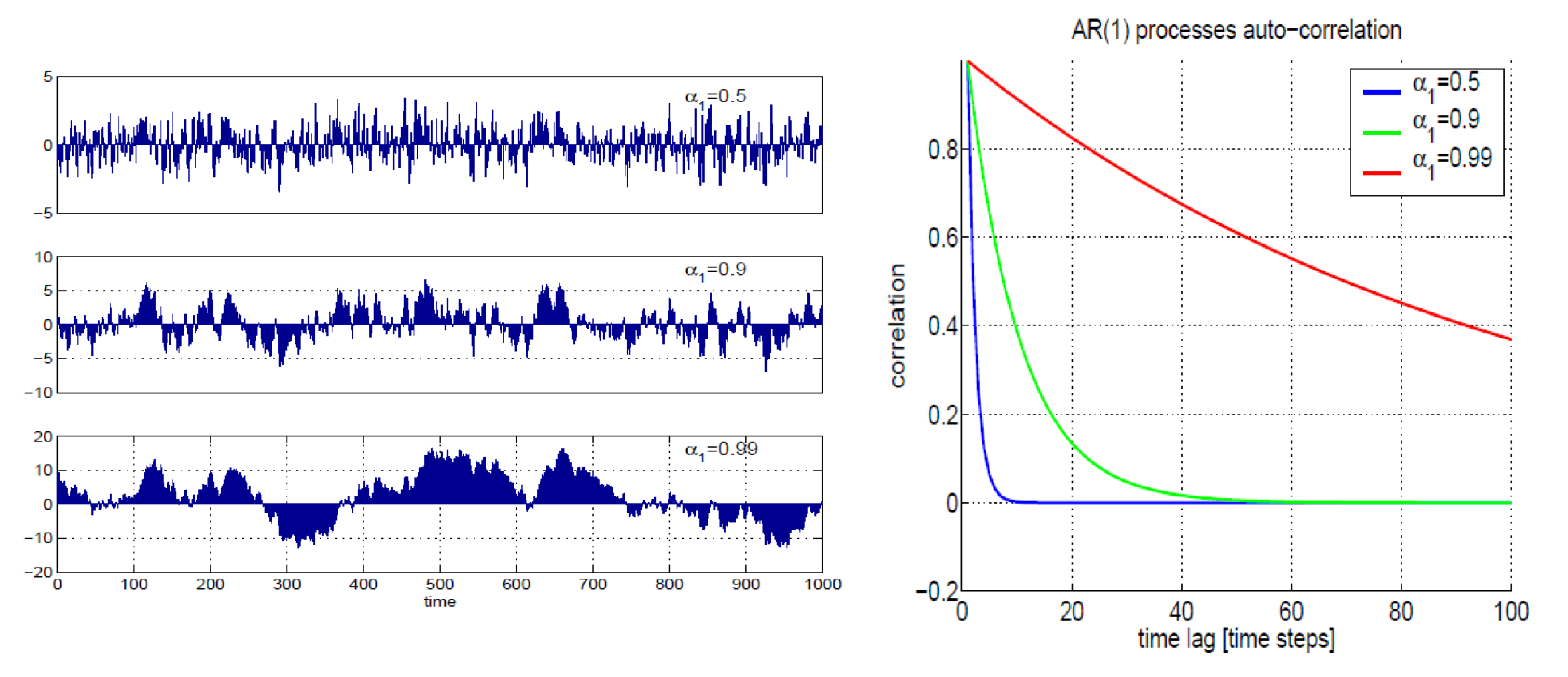
• auto-correlation functions of the above time series in Figure 3 below

Autoregressive (AR) processes

• in an AR process each value in a time series is modeled as a linear combination of its previous values, along with some random noise. a general AR(p) process can be represented as follows:

\[X_t = \alpha_1X_{t-1} + \alpha_2X_{t-2} + ... \alpha_pX_{t-p} + \varepsilon_t\]

\(\alpha_1,\alpha_2,...,\alpha_p\) - autoregressive coefficients determining the dependance on the past values,
\(\varepsilon_t\) - random error term or white noise at time \(t\)

• order p of the autoregressive process determines how many past values have to be considered in the predicition of the current value

• AR(1) processes rely only on the previous value

\[X_t = \alpha X_{t-1} + \varepsilon_t,\]

• while AR(2) processes rely on the previous two values

\[X_t = \alpha_1X_{t-1} + \alpha_2X_{t-2} + \varepsilon_t,\]

Decorrelation time

• describes characteristic timescales of stochastic processes: how fast the autocorrelation decreases with time lag as a measure of the memory and persistence of the processes

• number degree of freedom \(n_X\) of \(X\) (initially we had the definition for \(n_X\) that \(X_i\) and \(X_j\) have to be independent, meaning uncorrelated), central limit theorem:

\[Var(\mathbf{\bar{X}}) = \frac{\sigma^2_X}{n_X} \Rightarrow n_X\]

• relation between the true number of time steps used and \(n_X\) is the decorrelation time

\[\begin{split}\begin{align*} \tau_D &= \frac{n}{n_X}\\ &= 1+2\sum_{k=1}^{\infty}\rho(k),~~~~~\mathrm{for~ the~ mean}\\ &=1+2\sum_{k=1}^{\infty}\rho(k)^2,~~~\mathrm{for~ the~ variance} \end{align*}\end{split}\]