Climate of the Earth system

Prof. Dr. Markus Meier
Leibniz Institute for Baltic Sea Research Warnemünde (IOW)
E-Mail: markus.meier@io-warnemuende.de

Fundamental processes of the climate system

Earth’s climate system and its subsystems

Note

Definition of climate:
“Climate in a narrow sense is usually defined as the average weather, or more rigorously, as the statistical description in terms of the mean and variability of relevant quantities over a period of time ranging from month to thousands or millions of years. The classical period is 30 years, as defined by the World Meteorological Organization (WMO).”
(Houghton, J. T., et al. (eds.), 2001: Climate Change 2001: The Scientific Basis. Contribution of Working Group I to the Third assessment Report of the Intergovernmental Panel on Climate Change. Cambridge University Press, 881 p.) ```

Atmosphere:

• small heat capacity, fast response time to an imposed change

• time scales: annual cycle, synoptic activities (days to weeks), decadal variability; variations are called weather

Hydrosphere:

• covers ocean, lakes, rivers, precipitation, ground water

• ocean can be divided into the deep ocean (depth scale of 1000m with time scales of 100-1000 years) and the mixed layer (depth scale of 100m with time scales of weeks-months)

• high heat capacity, small albedo

Cryosphere:

• covers all ice and snow: inland glaciers of Greenland and Antarctica and other continental glaciers, snow fields, sea ice, permafrost

• high albedo, small thermal conductivity

• largest freshwater reservoir

• time scales from 1-10 years (sea ice) to 10\(^4\)-10\(^5\) years (inland ice)

Biosphere:

• terrestrial bio-geophysical interaction: albedo, evaporation, roughness

• terrestrial bio-geochemical interaction: photosynthesis and respiration of carbon, impact on CH\(_4\) emissions

• time scales ranging from minutes (physiology - reaction of the stomata) to 30-150 years (succession) to 300-1500 years (migration)

• marine biosphere acts as biological carbon pump, plays important role in carbon cycle and acts as CO\(_2\) sink/source

• time sclaes of marine biosphere similar to terrestrial ones

Pedosphere:

• outermost layer of the Earth composed of soils

• time scales of heat and water storage depend on the layer depth: daily cycle for depths of about 10-30cm and annual cycle for depths of a few metres

Lithosphere:

• crust and the upper Earth mantle

• important impact factors: orography, biogeochemistry (volcanoes)

• time scales of roughly 10\(^7\) years, i.e. formation of the Himalayas and the Alps ~ 10\(^6\) years, continental drift ~ 10\(^8\) years

Courtesy: U. Cubasch

Nice illustration of the processes inside the subsystems: Geomar Website

Radiation balance: deducing a simple climate model

Zero order model

• deduce a simplistic climate model based on a few assumptions and refine it step by step, therefore assuming Earth’s surface temperature as a scalar value instead of a scalar field, formulate radiation balance for surface temperature change depending on incoming solar radiation and outgoing thermal radiation

(1)\[\gamma \frac{dT_{surf}}{dt} = F_{solar} - F_{thermal}\]

\(\gamma\) - global surface heat capacity [\(J/m^2/K\)]
\(T_{surf}\) - global surface temperature [\(K\)]
\(F_{solar}\) - incoming solar radiation flux [\(W/m^2\)]
\(F_{thermal}\) - outgoing thermal radiation flux [\(W/m^2\)]

• zero order model for radiation balance (because T scalar), \(\gamma\) is important parameter, can be seen as heat capacity: scales temperature change due to difference in outgoing and incoming radiation, higher gamma means smaller temperature change for given \(\Delta F\) and vice versa

• solar constant \(S_0\) describes average solar radiation flux hitting earth, part of it is getting reflected due to Earth’s albedo. effectively only \(\pi r^2\) of total surface \(4\pi r^2\), so only \(\frac{1}{4}\) receives this radiation:

(2)\[F_{solar} = \frac{1}{4}S_0(1-\alpha_{surf})\]

\(S_0 = 1368 \frac{W}{m^2}\) - solar constant
\(\alpha_{surf} \approx 0.3\) - global surface albedo

• with very good approximity Earth can be seen as black body radiator, so outgoing radiation can be described by Stefan-Boltzmann law:

(3)\[F_{thermal} = \sigma T^4_{surf}\]

\(\sigma = 5.67 * 10^{-8} \frac{W}{m^2K^4}\) - Stefan-Boltzmann constant

• now assume balance between incoming and outgoing radiation on long term basis \(\rightarrow \frac{dT_{surf}}{dt}=0\):

\[\begin{split}F_{thermal} = F_{solar}\\\end{split}\]

• using the definitions of \(F_{solar}\) (2) and \(F_{thermal}\) (3):

(4)\[\begin{split}\sigma T^4_{surf} = \frac{1}{4}S_0(1-\alpha_{surf})\\\end{split}\]

• obtain expression for surface temperature solely on basis of radiation balance between insolation and thermal radiation

\[\Rightarrow T_{surf}^{0} = \sqrt[4]{\frac{S_0(1-\alpha_{surf})}{4 \sigma}} \approx 255K = -18°C\]

Greenhouse effect

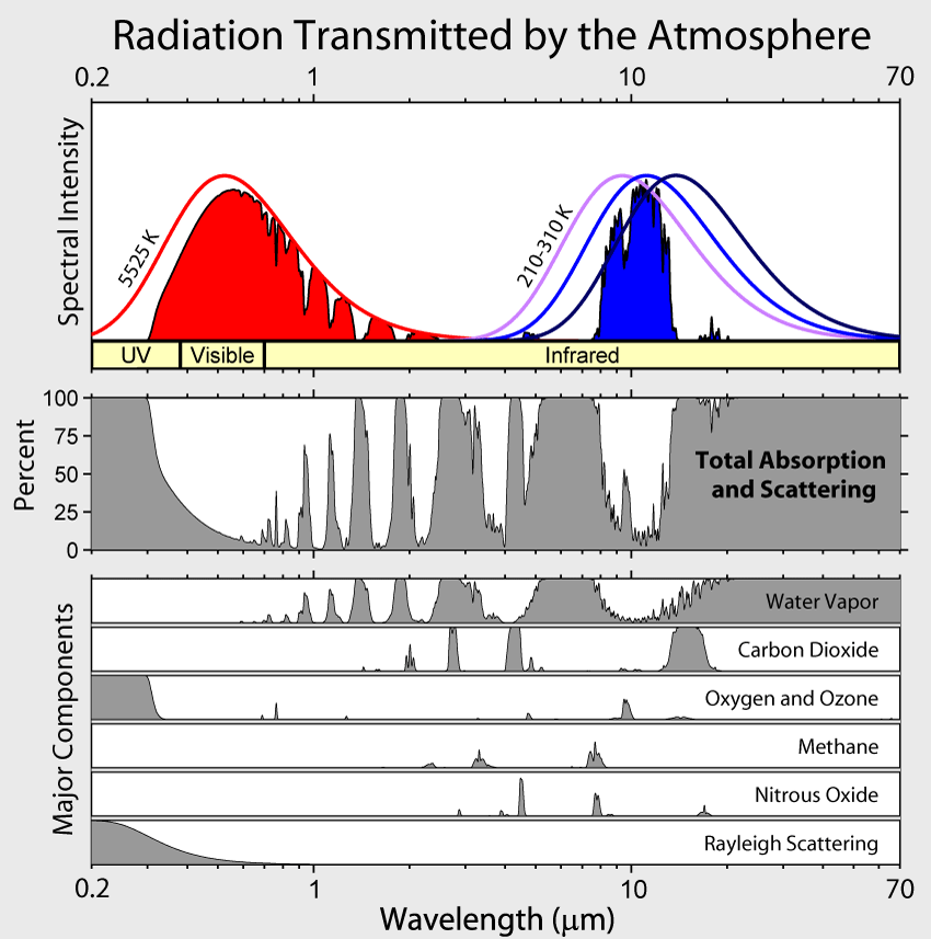
Fig. 2 Atmospheric absorption and scattering applied to the blackbody radiation spectra of sun and Earth

• atmosphere is mixture of many gases. main constitutients listed in table below. greenhouse gases are written in bold:

Atmospheric constitutient	Concentration by volume
Nitrogen (N\(_2\)	0.7808
Oxygen (O\(_2\))	0.2095
Argon (Ar)	0.0093
Carbon dioxide (CO\(_2\))	420 ppm (2023)
Neon (Ne)	18 ppm
Helium (He)	5 ppm
Methane (CH\(_4\))	1.9 ppm
Hydrogen (H\(_2\))	0.5 ppm
Nitrous oxide (N\(_2\)O)	0.3 ppm
Ozone (O\(_3\))	0-0.1 ppm

• below figure shows the influence of the planetary albedo and the greenhoouse effect happening in the atmosphere. solid line shows the blackbody radiation, meaning that the albedo is zero and all the solar radiation is absorbed and thermal radiation is emitted in an equilibrium. circle markers indicate the surface temperatures of the planets with their respective albedo – not all the insolation is absorbed, some is reflected , so that temperature is lower. star markers indicate the actual surface temperatures of the planets hich are strongly influenced by the greenhouse effect happening in the atmosphere of the planets. note how strong the effect is on Venus with a thick atmosphere and how weak on Mars with a very thin atmosphere.

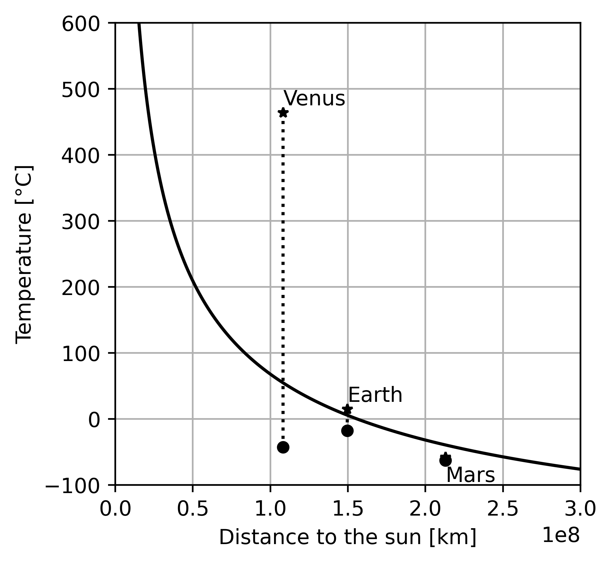
• actually \(T_{surf} \approx 15°C\), have to consider the role of Earth’s atmosphere, because greenhouse effect happens. most incoming solar radiation passes through atmosphere due too its short wavelength. outgoing thermal radiation with higher wavelengths is absorbed by the atmosphere and reemitted in all directions, also back to the surface. this implies that less energy escapes to space than what would be the case without an atmosphere. net effect is warming of the surface.

Greenhouse shield model

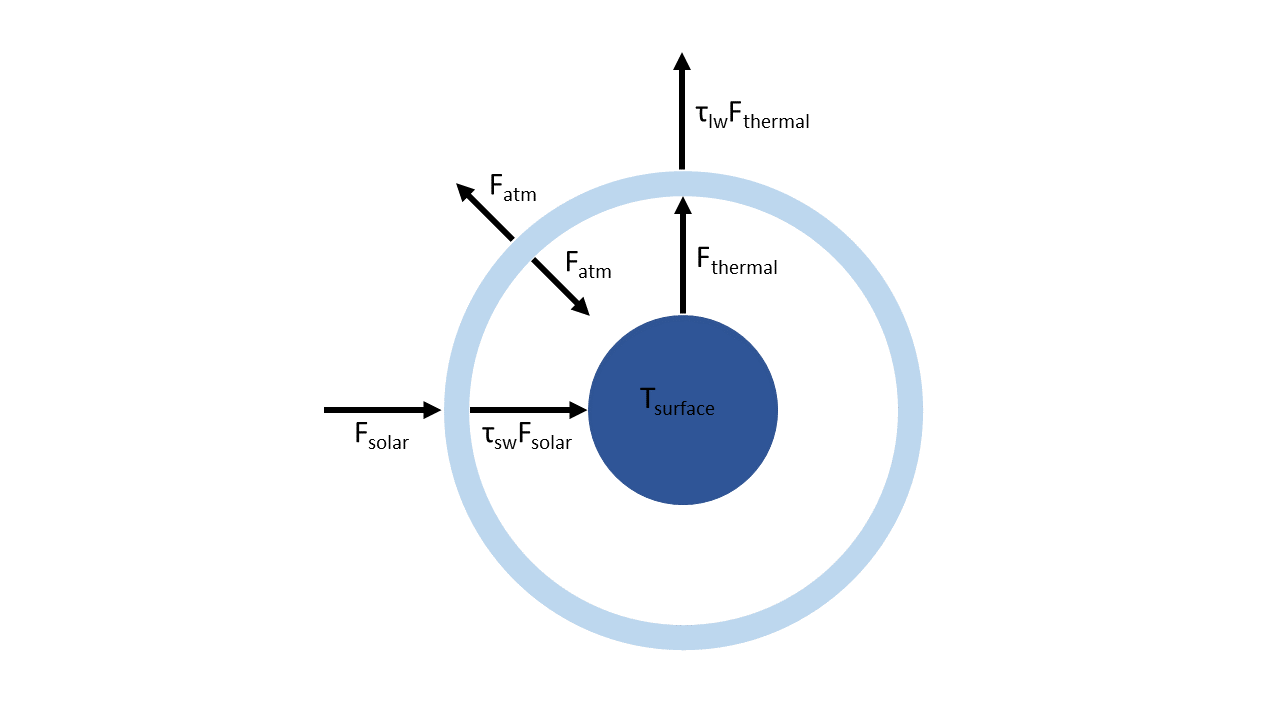
• can formulate radiation balances for top of atmosphere and Earth’s surface

(5)\[ \begin{align}\begin{aligned}\begin{split}\begin{align*} F_{solar} &= F_{atm} + \tau_{lw}F_{thermal}\\ \tau_{sw}F_{solar} + F_{atm} &= F_{thermal}\end{split}\\\end{align*}\end{aligned}\end{align} \]

\(\tau_{sw} \approx 0.67\) - atmospheric shortwave transmissivity
\(\tau_{lw} \approx 0.06\) - atmospheric longwave transmissivity

• can quickly eliminate \(F_{atm}\) from (5) to obtain:

(6)\[F_{solar} - \tau_{lw}F_{thermal} = F_{thermal} - \tau_{sw}F_{solar}\]

• which can be reframed to get:

\[F_{thermal} = F_{solar} \frac{1 + \tau_{sw}}{1 + \tau_{lw}}\]

• plugging in the definitions of \(F_{solar}\) (2) and \(F_{thermal}\) (3):

\[\sigma T_{surf}^4 = \frac{1}{4}S_0(1-\alpha_{surf}) \frac{1 + \tau_{sw}}{1 + \tau_{lw}}\]

• now we can get an expression for the surface temperature including the greenhouse effect:

\[T_{surf}^1 = \sqrt[4]{\frac{1}{4\sigma}S_0(1-\alpha_{surf}) \frac{1 + \tau_{sw}}{1 + \tau_{lw}}} \approx 285K = 12°C\]

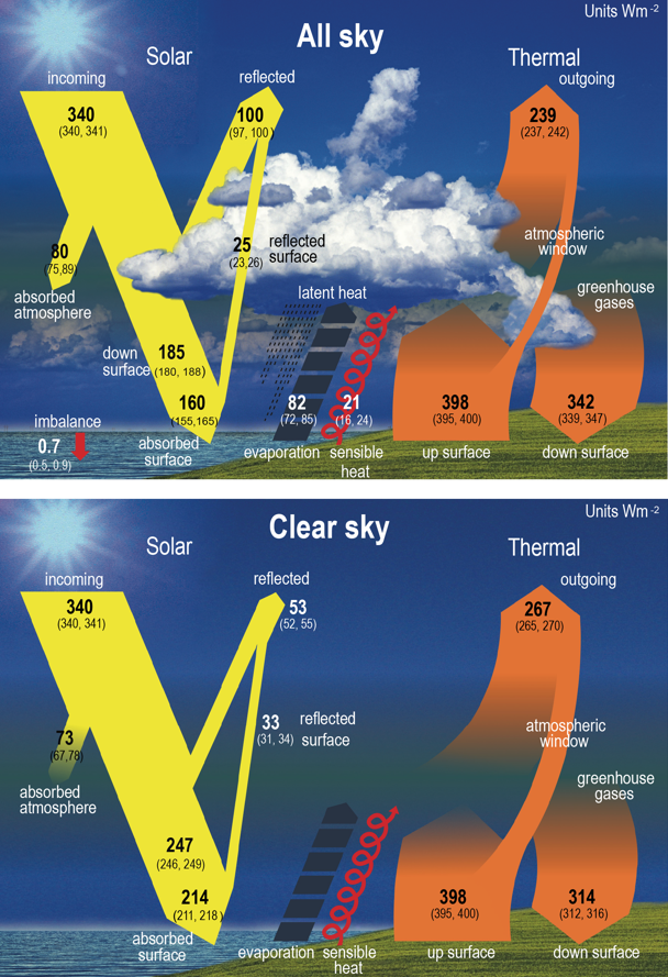
• albedo = solar incoming/solar reflected = 100/340 = 0.29

• imbalance = 0.7 \(\frac{W}{m^2}\)

• absorbed by surface = absorbed surface/solar incoming = 160/340 = 0.47

• atmospheric shortwave transmissivity \(\tau_{sw}\) = absorbed surface/(solar incoming - solar reflected) = 160/(340-100) = 0.67

• atmospheric longwave transmissivity \(\tau_{lw} \approx\) 0.06, see atmospheric window

Greenhouse model with ice-albedo feedback

• net absorbed energy of \(0.7\frac{W}{m^2}\) -> warming. warming means melting of ice and snow -> albedo decreases (see below values, difference from ice and snow to water): this is the ice-albedo feedback

Properties of the ground	Albedo [%]
Snow	75-95
Old snow	50-70
Ice	30-40
Sand	20-30
Grass	15-20
Forest	5-20
Water	3-10
Water (with sun close to the horizon)	10-100

• idea of Budyko 1969 to implement ice-albedo feedback into the zero order model with thee greenhouse effect. start from zero order model (1):

(7)\[\gamma \frac{dT_{surf}}{dt} = \frac{S_0}{4}(1-\alpha_{feedback}) - F_{thermal}\]

• adapt two things: 1. linearize earths thermal radiation \(F_{thermal}\) and include the greenhouse effect in the parameters and 2. formulate earths albedo \(\alpha\) as a function of T_surf

• 1: linearize thermal radiation as a function of surface temperature:

(8)\[F_{thermal} = A + B*(T_{surf} - 273.15K)\]

\(A = 203.3 \frac{W}{m^2}\)
\(B = 2.09 \frac{W}{m^2K}\)

• values for A and B taken from observations so they include the greenhouse effect

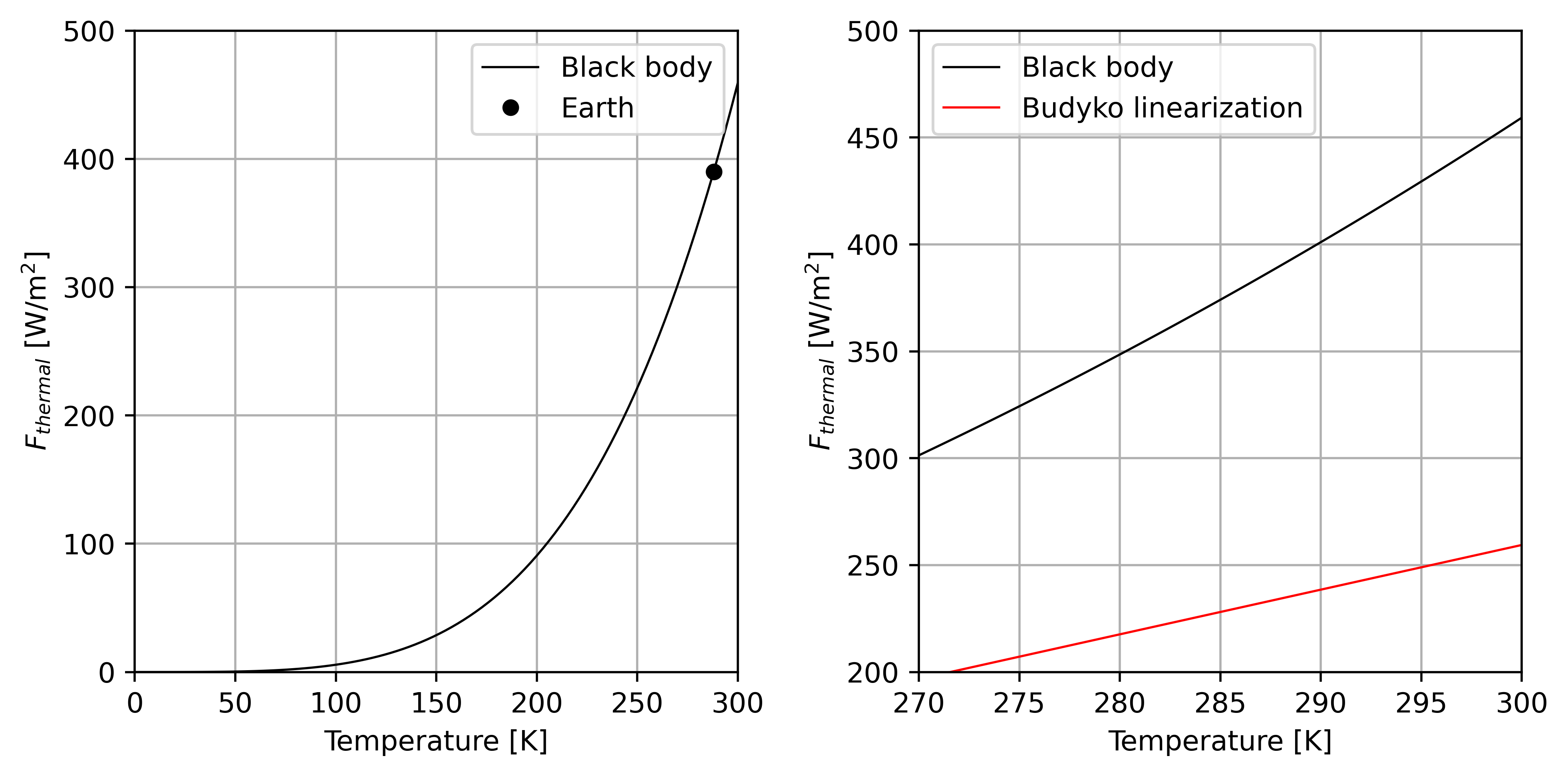
• see that linearization in red is a good approach and see that linearization parameter B includes greenhouse effect as red slope is smaller than black slope

• 2: now we want to describe albedo \(\alpha\) as a function of \(T_{surf}\) instead of setting a constant value

• there are two extremes: a totally ice-covered world with the albedo \(\alpha_{ice} = 0.62\), we assign that to be the case for temperatures lower than \(T_{ice}=-10°C\). or a totally ice free world with an albedo of \(\alpha_{noice} = 0.30\) for temperatures over \(T_{noice}=0°C\). for temperatures in between assume a linear decrease of the albedo:

(9)\[\begin{split}\alpha_{feedback}(T_{surf})= \left\{ \begin{array}{ll} \alpha_{ice} & T_{surf}<T_{ice} \\ \alpha_{ice} - \frac{0.32}{10K}(T_{surf}-T_{ice}) & T_{ice} < T_{surf} < T_{noice}\\ \alpha_{noice} & T_{noice} < T_{surf}\\ \end{array} \right.\end{split}\]

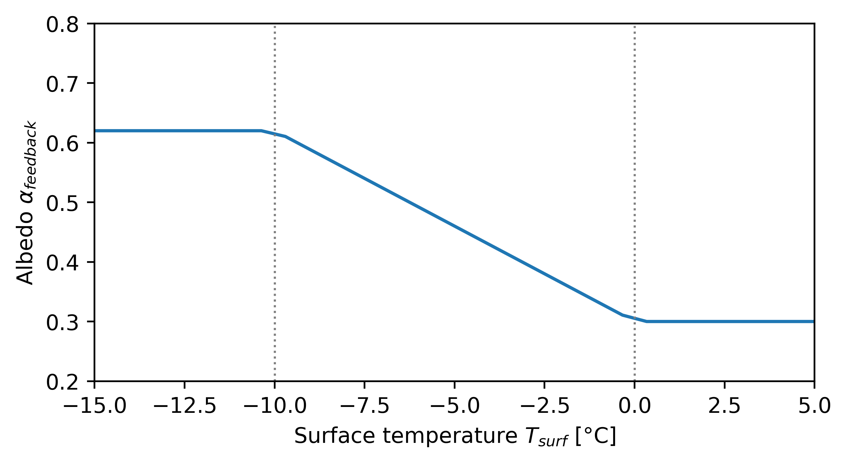
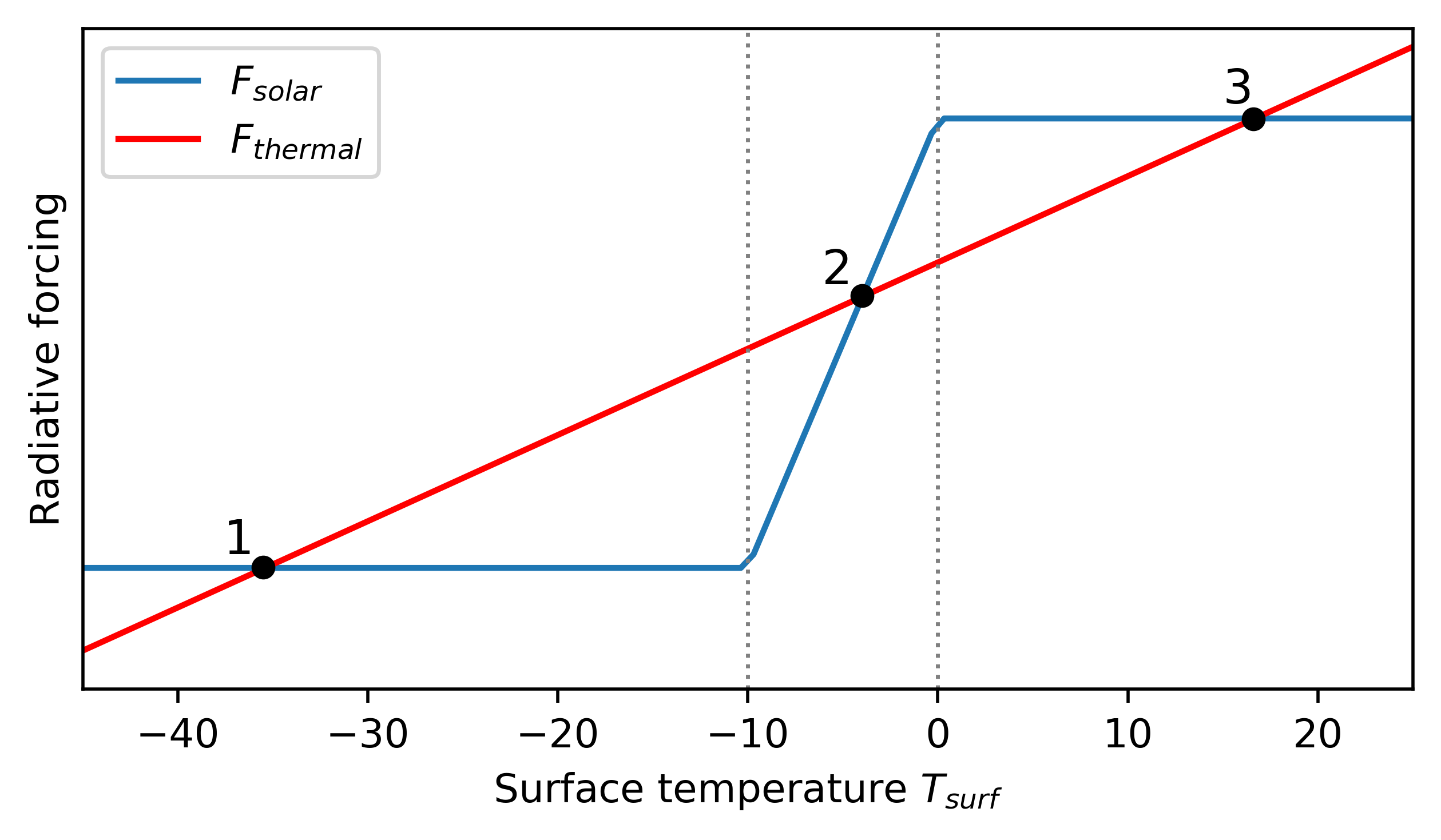
• in order to get equilibrium surface temperatures we set \(\frac{dT_{surf}}{dt}=0\) and insert (8), and (9) into (7). this yields:

(10)\[\frac{S_0}{4}(1-\alpha_{feedback}) = A + B*(T_{surf} - 273.15K)\]

• equation has three solutions all representing an equilibrium state for the surface temperature:

\[\begin{split}\begin{align*} &\textrm{1. fully ice covered Earth:}~~~~~~~~~~T_{surf} = \frac{(1-\alpha_{ice})S_0/4-A}{B} +273.15K= -35.4°C\\ &\textrm{2. partially ice covered Earth:}~~~T_{surf} = \frac{\frac{S_0}{4} \left( 1-\alpha_{ice} -\frac{0.32}{10°C}T_{ice}\right)-A}{B-\frac{S_0}{4}\frac{0.32}{10K}} +273.15K = -4.0°C\\ &\textrm{3. Earth without ice cover:}~~~~~~~~T_{surf} = \frac{(1-\alpha_{noice})S_0/4-A}{B} +273.15K = 16.7°C \end{align*}\end{split}\]

Climate stability and sensitivity

Climate potential

• what happens when deviation from these equilibrium temperatures? in general there are two types of equilibria: if adding a small perturbation to a stable equilibrium it returns to its initial state. if adding a small perturbation to an unstable equilibrium the perturbation starts growing and the system will not return to equilibrium state- it will drift away

• for climate science a climate potential P describes these behaviours. P is defined as:

(11)\[P(\chi) = - \int F_{total}(\chi)~d\chi,\]

• in our case of the greenhouse model with ice-albedo feedback: \(\chi\) the variable of interest that the potential depends on, \(T_{surf}\); and \(F_{total}\) the forcing on the system, for us \(F_{solar}-F_{thermal}\). insert into (11):

(12)\[\begin{split}\chi \rightarrow T_{surf}\\ F_{total}(\chi) \rightarrow F_{solar}(T_{surf})~-~F_{thermal}(T_{surf})\\ P(T_{surf}) = -\int F_{solar}-F_{thermal} ~dT_{surf}\end{split}\]

• recalling the definitions of \(F_{solar}\) and \(F_{thermal}\) yields formula for the climate potential of the greenhouse model with ice-albedo feedback:

(13)\[\begin{split}\begin{align*} P(T_{surf}) &= -\int \left( \frac{S_0}{4}(1-\alpha_{feedback}(T_{surf})) - (A + B(T_{surf}-273.15K)) \right)~ dT_{surf}\\ &= AT_{surf} + B \left( \frac{1}{2}T_{surf}^2- T_{surf}*273.15K\right)-\frac{S_0}{4} \int (1-\alpha_{feedback}(T_{surf}))~dT_{surf} \end{align*}\end{split}\]

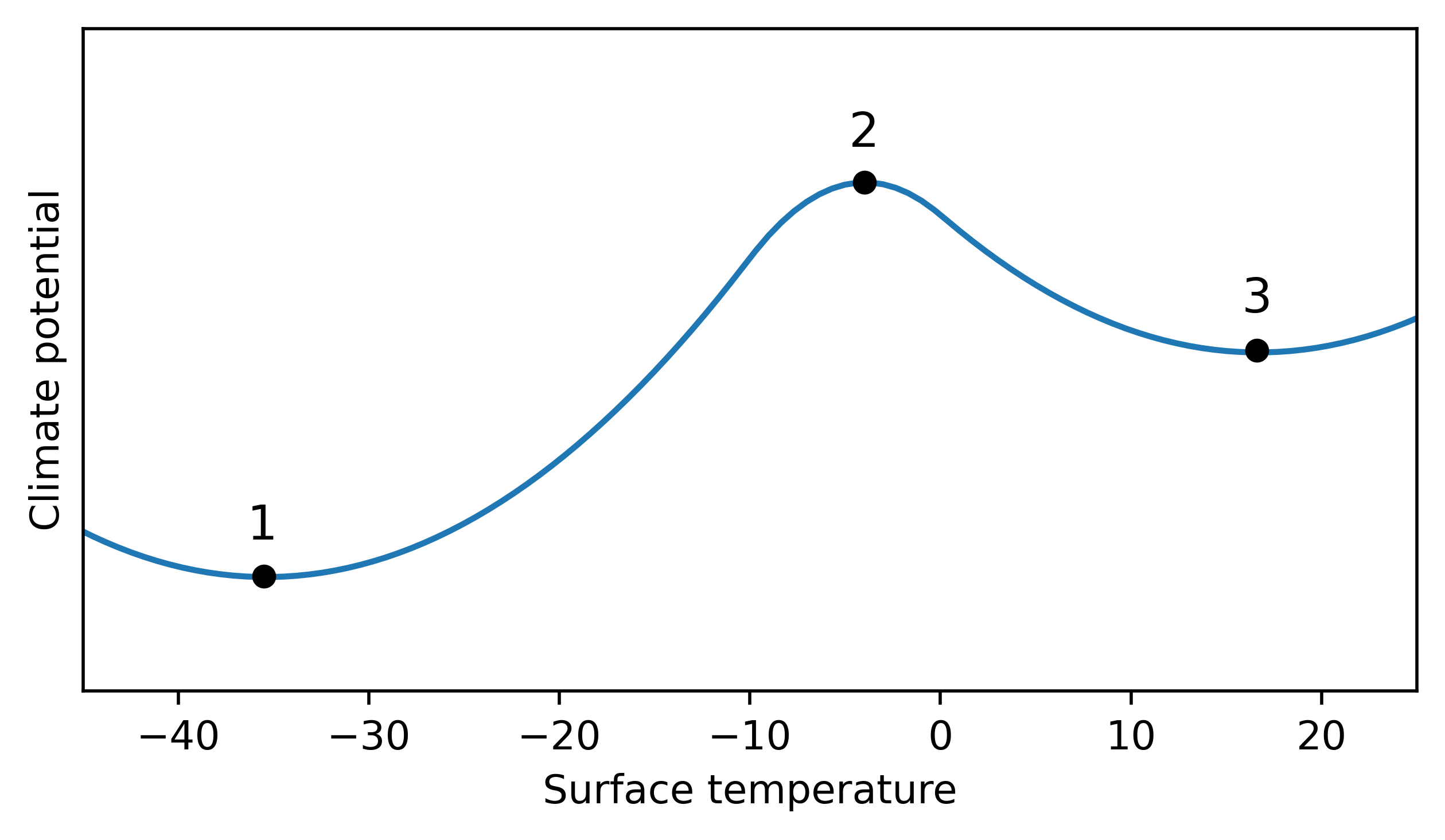
• recalling the definition of the potential (11) we can describe the forcing of our climate system if the climate potential is known as:

(14)\[F_{total}(T_{surf}) = -\frac{dP(T_{surf})}{dT_{surf}}\]

• apply this definition to climate potential shown in Figure 10. in point 1: perturbation to left/right cause force in opposite direction, back to equilibrium. same for point 3. but perturbing the system from point 2 causes a force in the same direction, away from the equilibrium.

  1. Totally ice covered earth is stable.

  2. Partially ice covered earth is unstable.

  3. Earth without ice cover is stable.

Tipping points of the climate system

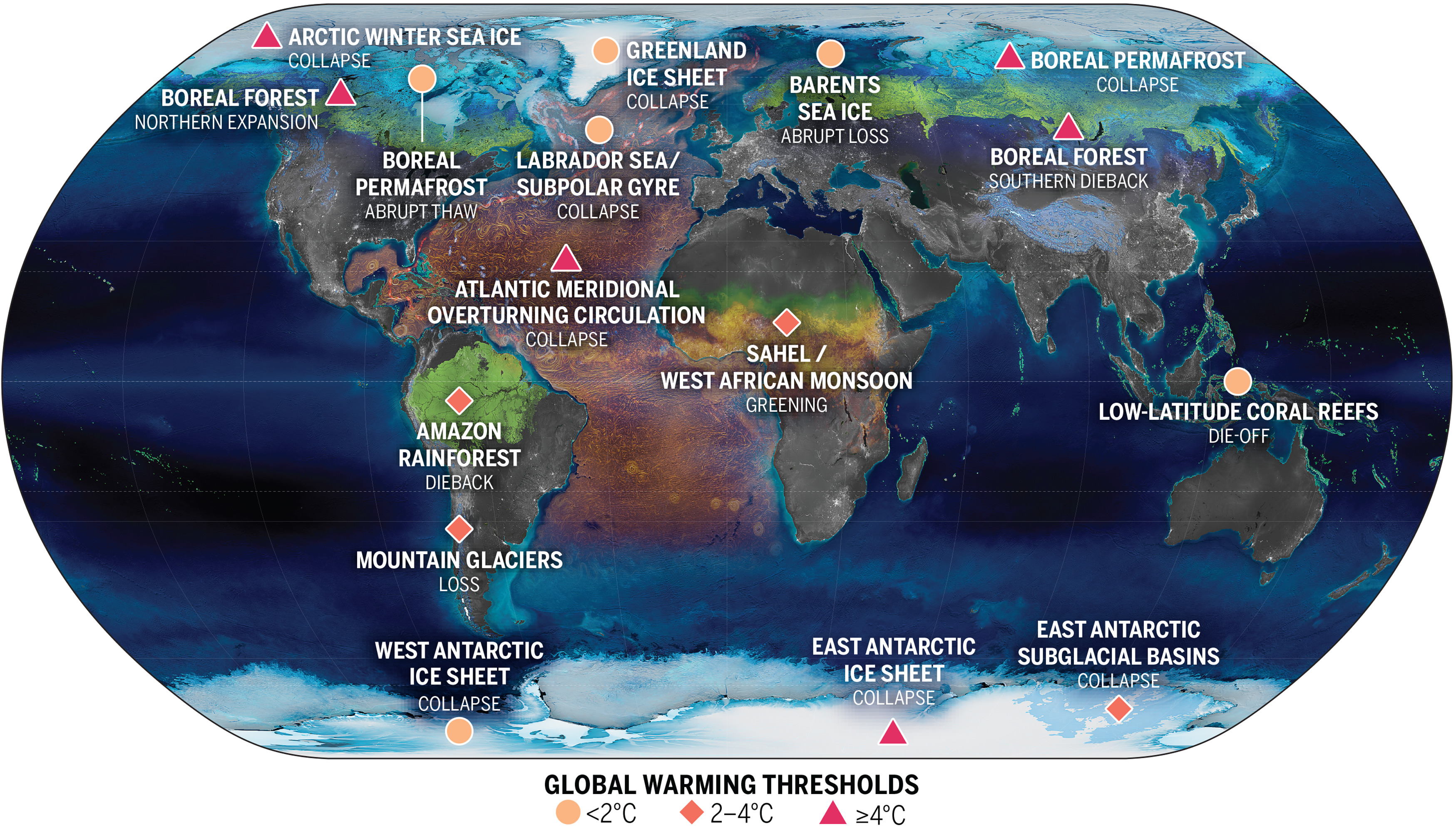
• tipping point is a criticial threshold beyond which a small change can cause strong and often times irreversible changes to the climate system. figure 11 shows the most important known tipping points of our climate system.

• tipping point is described by a local maximum of the climate potential. if an additional constant forcing \(C\) is added to the total forcing in equation (12):

(15)\[P(T_{surf}) = -\int (F_{solar} - F_{thermal} + C)~dT_{surf},\]

• we obtain

\[P(T_{surf}) = P_0(T_{surf}) - CT_{surf},\]

• with the original potential

(16)\[P_0(T_{surf}) = -\int (F_{solar}-F_{thermal}) ~dT_{surf}.\]

• constant additional forcing effectively rotates the potential clockwise

• imagine ball in the modified potential rolling into new equilibrium

• after removing the additional forcing to return to the potential \(P_0\): system is still in new equilibrum state -> climate change is irreversible!

Climate sensitivity

• describes the change of temperature or any other variable of interest per change in forcing. forcing can be different things, such as forcing through carbon emissions, a change in solar forcing, volcanic eruptions, many more. we look at

(17)\[\lambda = \frac{\Delta T}{\Delta Q}\]

• for our different climate models from 2.2.

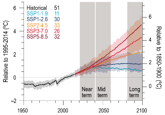
• 1. IPCC AR6 from 2021 gives different climate change scenarios called SSP… (Shared Socioeconomic Pathways), shown in figure 14. last number of these pathways indicate the additional radiative forcing. for SSP1-2.6: \(\Delta Q = 2.6 \frac{W}{m^2}\) with a temperature change relative to preindustrial time of \(\Delta T = 2K\). inserting these 2 values into (17):

(18)\[\lambda_1 = \frac{2.0K}{2.6 \frac{W}{m^2}} = 0.77 \frac{m^2K}{W}\]

• 2. zero order model. use equation (30). Q is absorbed solar radiation \(Q=F_{solar}\).

  \[\lambda_2 = \frac{dT_{surf}}{dQ} = \frac{d}{dQ} \left[ \left( \frac{Q}{\sigma} \right)^{\frac{1}{4}} \right] = \frac{1}{4\sigma} \left( \frac{Q}{\sigma} \right)^{\frac{-3}{4}} = \frac{\left( \frac{Q}{\sigma} \right)^{\frac{1}{4}}}{4Q} = \frac{T_{surf}}{4Q} = \frac{255K}{4*239.4\frac{W}{m^2}} = 0.27 \frac{m^2K}{W}\]

• 3. Greenhouse shield model. using (10) and noting that the left side is just \(F_{solar}\), which is our Q:

  \[\lambda_3 = \frac{dT_{surf}}{dQ} = \frac{d}{dQ} \left( \frac{Q -A}{B} -273.15K \right) = \frac{1}{B} = 0.48 \frac{m^2K}{W}\]

• 4. Greenhouse model with ice-albedo feedback. interesting part is where the world is partially ice covered and the feedback mechanism happens. but previous calculations revealed unstable equlibrium in this area. it doesnt make sense to analyse cliate sensititvity around unstable points. small perturbations cause high temperature changes which are not actually caused by the change in forcing but by the system falling into a new equilibrium. if we reduce the albedo gradient from \(-0.032\frac{1}{K}\) to \(-0.003\frac{1}{K}\). furthermore we assume \(Q = \frac{S_0}{4}\), so that the effects of the albedo feedback can be noticed. we can rewrite (10):

  \[Q(1-\alpha_{ice} + 0.003\frac{1}{K}(T_{surf}-T_{ice}) = A + B(T_{surf} +273.15K)\]

• rewriting this expression for \(T_{surf}(Q)\) (can be done as homework) yields:

  \[\lambda_4 = \frac{dT}{dQ} = 0.66 \frac{m^2K}{W}\]

• ice-albedo feedback increases climate sensitivity drastically.

Feedback mechanisms

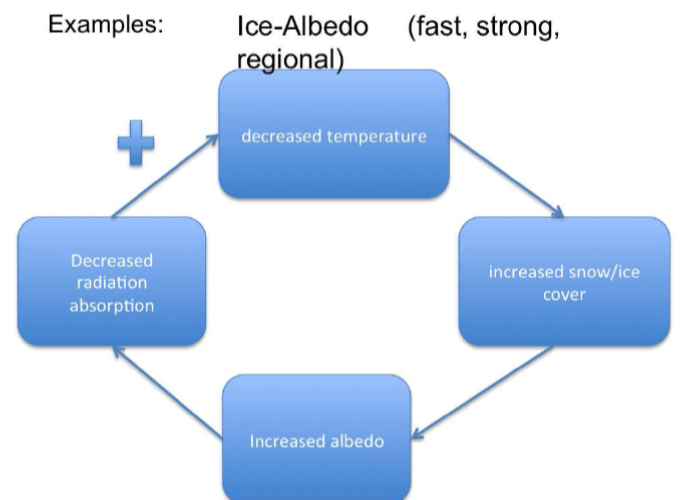
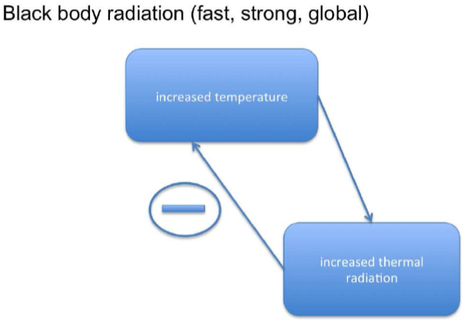
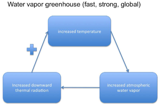
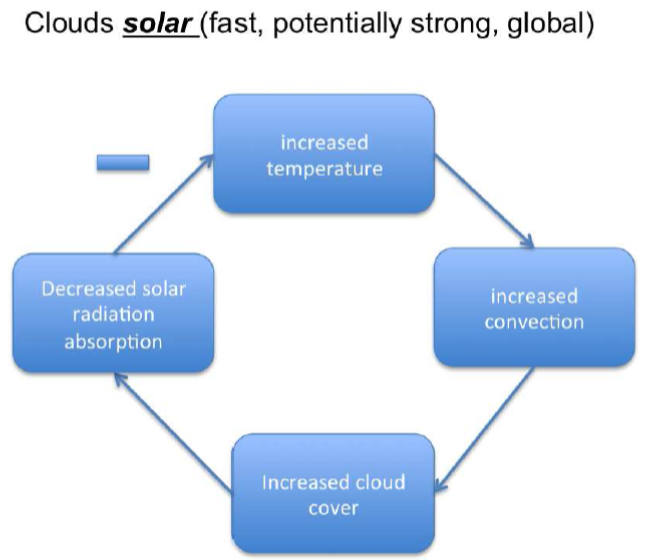
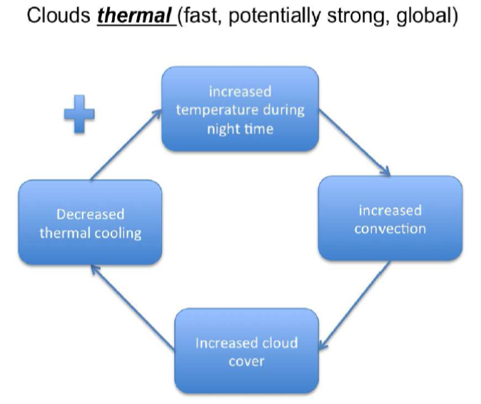
• in general we have climate system Earth and look at the temperature. change in temperature can trigger two different kinds of feedback. first a positive feedback, which is a reaction of the system to the change in temperature, that further increases the trend. negative feedback is the opposite: the system reacts to a change in temperature in a way opposing the original trend thus decreasing it. lets go through a few examples:

1. ice-albedo feedback: temperature increases which causes the melting of surface ice, which increases the planetary albedo which leads to an increase in absorbed solar radiation.

Courtesy: D. Dommenget

Questions:

1. Explain what an Earth system approach is. Which are the five components of the Earth climate system? Provide brief characteristics.

2. List three important greenhouse gases.

3. Explain the greenhouse effect in detail.

4. Define climate feedbacks and climate sensitivity and relate the two quantities to each other. Explain at least one example of a climate feedback.

5. What is a tipping point of the climate system? (Hint: draw a sketch of a climate potential and explain in words why changing climate might be irreversible.)

Table of figures

Figure 1: FAQ 1.2, Figure 1 in IPCC, 2007: Chapter 1. In Climate Change 2007: The Physical Science Basis. Contribution of Working group I to the Fourth Assessment Report of the Intergovernmental Panel on Climate Change [Core Writing Team, Pachauri, R.K. and Reisinger, A. (eds.)]. IPCC, Geneva, Switzerland, 104pp. Figure 2: https://www.geomar.de/en/discover/ocean-and-climate/model-simulations/the-earths-climate-system, access on 22.02.2024 Figure 3: Robert A. Rohde, https://commons.wikimedia.org/wiki/File:Atmospheric_Transmission.png, access on 24.02.2024, GNU Free Documentation License Figure 6: IPCC, AR6 Climate Change 2021: The Physical Science Basis. Contribution of Working Group I to the Sixth Assessment Report of the Intergovernmental Panel on Climate Change [Forster, P., T. Storelvmo, K. Armour, W. Collins, J.-L. Dufresne, D. Frame, D.J. Lunt, T. Mauritsen, M.D. Palmer, M. Watanabe, M. Wild, and H. Zhang, 2021: The Earth’s Energy Budget, Climate Feedbacks, and Climate Sensitivity. In Climate Change 2021: The Physical Science Basis. Contribution of Working Group I to the Sixth Assessment Report of the Intergovernmental Panel on Climate Change [Masson-Delmotte, V., P. Zhai, A. Pirani, S.L. Connors, C. Péan, S. Berger, N. Caud, Y. Chen, L. Goldfarb, M.I. Gomis, M. Huang, K. Leitzell, E. Lonnoy, J.B.R. Matthews, T.K. Maycock, T. Waterfield, O. Yelekçi, R. Yu, and B. Zhou (eds.)]. Cambridge University Press, Cambridge, United Kingdom and New York, NY, USA, pp. 923–1054, doi: 10.1017/9781009157896.009 .]
Figure 11: D. I. Armstrong McKay et. al.. Exceeding 1.5°C global warming could trigger multiple climate tipping points. Science, Vol. 377, Issue 6611, 2022. https://doi.org/10.1126/science.abn7950 Figure 14: Figure 1.16 in IPCC, 2021: Chapter 1. In: Climate Change 2021: The Physical Science Basis. Contribution of Working Group I to the Sixth Assessment Report of the Intergovernmental Panel on Climate Change [Chen, D., M. Rojas, B.H. Samset, K. Cobb, A. Diongue Niang, P. Edwards, S. Emori, S.H. Faria, E. Hawkins, P. Hope, P. Huybrechts, M. Meinshausen, S.K. Mustafa, G.-K. Plattner, and A.-M. Tréguier, 2021: Framing, Context, and Methods. In Climate Change 2021: The Physical Science Basis. Contribution of Working Group I to the Sixth Assessment Report of the Intergovernmental Panel on Climate Change [Masson-Delmotte, V., P. Zhai, A. Pirani, S.L. Connors, C. Péan, S. Berger, N. Caud, Y. Chen, L. Goldfarb, M.I. Gomis, M. Huang, K. Leitzell, E. Lonnoy, J.B.R. Matthews, T.K. Maycock, T. Waterfield, O. Yelekçi, R. Yu, and B. Zhou (eds.)]. Cambridge University Press, Cambridge, United Kingdom and New York, NY, USA, pp. 147–286, doi: 10.1017/9781009157896.003 .]