Climate of the Earth system

Prof. Dr. Markus Meier
Leibniz Institute for Baltic Sea Research Warnemünde (IOW)
E-Mail: markus.meier@io-warnemuende.de

Climate models

• Types of climate models:

  1. Energy Balance Models (EBMs): Based on a radiation balance between Sun and Earth, remember lecture 2.

  2. Single-Column Models (SCMs): Analysing the atmosphere as a single vertical column. So the horizontal structure is neglected and the focus lies on the vertical structure.

  3. General circulation models (GCMs): Modeling ocean or atmosphere or both (coupled GCM) in 3D on a global scale. Different GCMs implement a different amount of characteristic processes of the climate system.

  4. Regional climate models (RCMs): Modeling the climate for a certain region, i. e. the Baltic Sea region. They can account for regional features such as coastal effects or topography and generally operate on a higher resolution than GCMs.

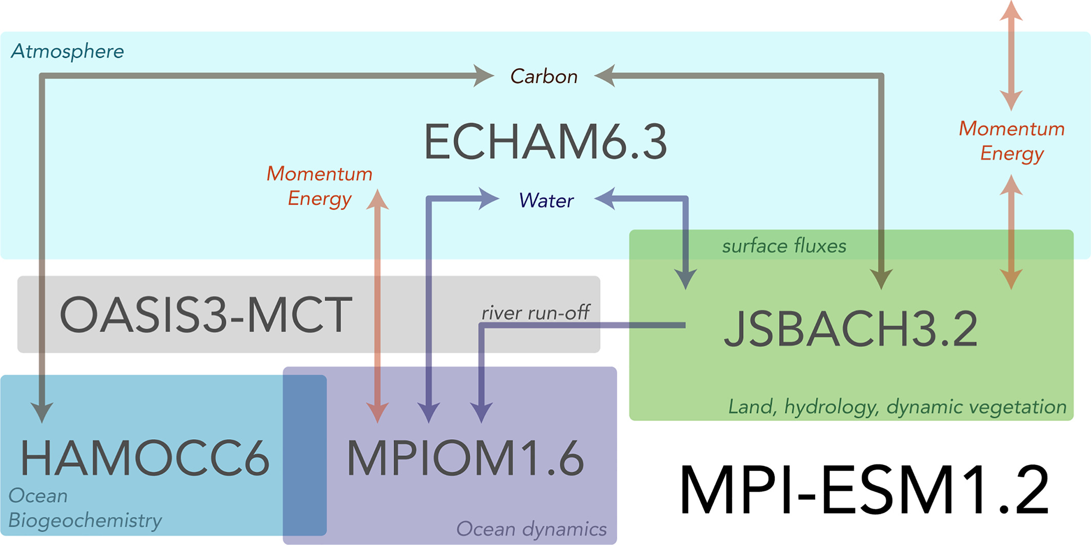
  5. Earth System Models (ESMs): Even more refined than GCMs incorporating more processes, generally coupling different sub-models. Covering all components of the climate system: Atmosphere, Hydrosphere, Cryosphere, Lithosphere, Biosphere, Pedosphere.

Courtesy: B. Rose

Running a GCM

• Model describing the General Circulation of the atmosphere and ocean. In a GCM latitude-longitude grid boxes cover the whole Earth over vertical levels in ocean and atmosphere.

Spatial and temporal resolution

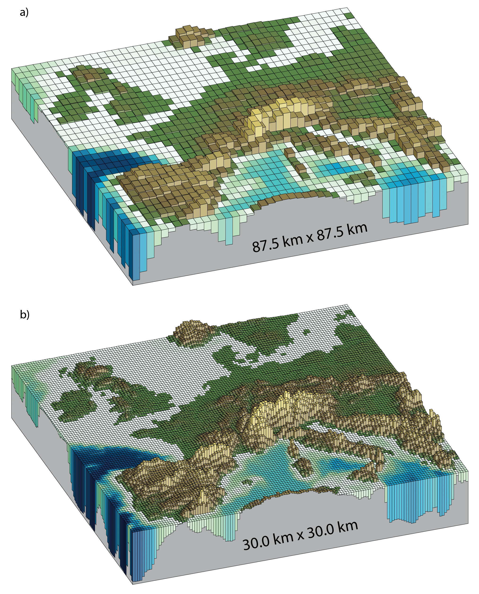
• Typical resolutions are 100-400km horizontally with 20-40 vertical levels and time steps of around 30min.

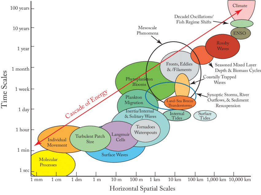
• Physical processes take place on different temporal and spatial scales. Difficulty lies in resolving them. If the model resolution is coarser than temporal or spatial scale of a process, this process cannot be resolved by the model!

• Processes on all scales interact with each other

• Of course we want to make the grid cells as small as possible, but there is always the trade-off between resolution and computational effort. As a result ocean and atmosphere models have less degrees of freedom than the real ocean/atmosphere, because it is impossible to include processes of all length scales so the focus is put on the longest scales (which carry most energy annd momentum).

General procedure

• Now we have chosen appropriate grid spacing and time evolution discretization. So let’s go, we can run the model as follows:

  1. Start from a given state of the climate system: Initialize each box for each state variable (temperature, pressure and many more)

  2. Calculate time tendencies of the state variables based on their current configuration (simply put: the temperature of this box will increase because all of the surrounding boxes are much warmer -> heat flux through the boundaries of the box)

  3. Add the calculated tendencies to the state of the system (these are the new temperature, pressure, etc. of this box)

  4. Derive new tendencies, add to the state etc.

• So far so easy. But their are two important remaining questions to be answered:

  • Which initial state should be chosen? The initial state has a crucial impact for the entire integration. Remember deterministic chaos.

  • How do we actually compute the tendencies in 2.? This is where the physics happens.

Ensemble runs

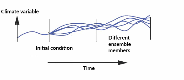
• A common method to acheive results that are least influenced by the inner variability of the system are ensemble runs. If a model is run from slightly differing initial states the outcome can be totally different due to the internal variability of the system. This variability is an important feature of the climate system, not only in models but in the real world. In order to obtain the tendencies of the model an ensemble of runs with slightly different initial conditions are performed and averaged.

• The problem of the initialization of the model is solved. Now let’s dive into the time propagation.

Time propagation

• Large-scale circulation models for ocean and atmosphere solve the dicretized (\(\frac{dT}{dt} \rightarrow \frac{\Delta T}{\Delta t}\)) primitive equations for each time step: a system of non-linear partial differential equations for salinity, potential temperature and velocity plus an equation of state. They are derived from conservation principles for mass, salinty and momentum and the first and second law of thermodynamics.

• For example a box has a given temperature. Now the temperature tendency for the box \(\Delta T\) (along with the tendencies of all other state variables for all boxes) is computed by solving the discretized primitive equations for a given time step. Adding the temperature tendency onto the previous temperature of the box yields the new temperature after the time step. This is done again and again until the time is propagated as wanted.

Add explanation for following images 7-9:

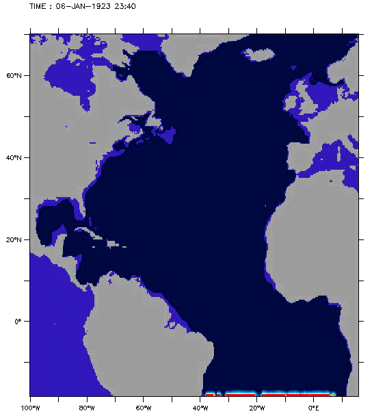
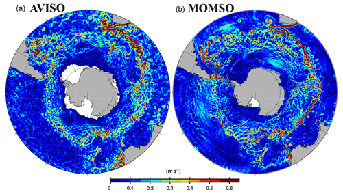
General problems of climate models

1. Useful models must be simpler than the real atmosphere/ocean.

• Time propagation is based on the primitive equations. These are derived from the Navier-Stokes equations using approximations which are carried into the model. That way the problem is simplified while retaining key physical phenomena:

  • Hydrostatic approximation:
    Eliminates vertical acceleration terms by assuming \(\frac{dp}{dz}=-\rho g\)

  • Traditional approximation:
    Neglecting coriolis terms in the horizontal momentum equations involving the vertical velocity and smaller metric terms.

  • Shallow-water approximation:
    Assuming that the depth of the ocean is small compared to the scale of characteristic processes.

  • Boussinesq approximation for the ocean:
    Eliminates sound waves while still accounting for buoyancy. It assumes that the ocean density is constant except in the buoyancy term, where small density differences play a significant role.

• Another commonly applied method is the Reynolds averaging of the primitive equations:

  • Reynolds averaging:
    Separating the flow variables (i.e. \(u,p,\rho\)) into mean values (i.e. \(\bar{u},\bar{p},\bar{\rho}\) representing the large-scale flow and fluctuating values (i.e. \(u',p',\rho'\)) representing the turbulence, and then time-averaging on a time scale large enough to filter out the turbulence but small enough to preserve the large-scale flow field.

2. Discrete equations are not the same as continous equations (calculation error).

• The only way to solve the primitive equations (set of non-linear differential equations) is to discretize them and solve them numerically. The discretization happens on temporal and spatial scale: vertical columns of latitude-longitude boxes for which all variable values get updated each time step \(\Delta t\). The discretizations are derived from the Taylor-series expansions. Let’s look at the pressure as a fuction of time \(p(t)\) as an example. Taylor expansion around \(p(t)\). A forward time step is given as:

(22)\[\begin{split}p(t+\Delta t) &= p(t) + \Delta t \frac{\partial p(t)}{\partial t} + \frac{1}{2} \Delta t^2 \frac{\partial^2 p(t)}{\partial t^2} + ...\\\end{split}\]

• and a backward time can be described by:

(23)\[\begin{split}p(t-\Delta t) &= p(t) - \Delta t \frac{\partial p(t)}{\partial t} + \frac{1}{2} \Delta t^2 \frac{\partial^2 p(t)}{\partial t^2} - ...\\\end{split}\]

• The two expansions (22) and (23) can be processed differently to different gain schemes approximating \(\frac{\partial p(t)}{\partial t}\). Rewriting the expansion (22) up to the first-order term \(+\Delta t \frac{\partial p(t)}{\partial t}\) yields:

\[\frac{\partial p}{\partial t} = \frac{p(t+\Delta t) - p(t)}{\Delta t}+\mathcal{O}(\Delta t^2)~~(\mathrm{forward~difference~scheme})\]

• Rewriting the expansion (23) up to the first-order term \(-\Delta t \frac{\partial p(t)}{\partial t}\) yields:

\[\frac{\partial p}{\partial t} = \frac{p(t) - p(t-\Delta t)}{\Delta t}+\mathcal{O}(\Delta t^2)~~(\mathrm{backward~difference~scheme})\]

• Substracting the two expansions results in:

\[\frac{\partial p}{\partial t} = \frac{p(t+\Delta t) - p(t-\Delta t)}{2\Delta t}+\mathcal{O}(\Delta t^2)~~(\mathrm{central~difference~scheme})\]

• There are other methods to describe the first derivative with higher-order accuracy.

• Derivatives with repsect to other variables are discretized in the same way. For higher-order derivatives schemes with different accuracies (leading order error term) can be deployed. The simplest example can be be deduced adding our two Taylor-expansions (22) and (23). The result is called the three-point-stencil, because the value of the second derivative is given by the values of three points:

\[\frac{\partial^2 p(t)}{\partial t^2} = \frac{p(t+\Delta t)-2p(t) + p(t-\Delta t)}{\Delta t^2}\]

• There are many more funky tools to navigate the numerical solution of differential equations. The lecture Computational Quantum and Many-Particle Physics facilitates a deeper dive into the topic.

• Inevitably the discretization introduces several errors to the numerical output of the model:

  • Truncation error: The Taylor-expansions which build the foundation of the schemes have to be truncated at some point. Above we did it after the first-order and neglected all higher-order terms. This truncation inevitable leads to an error in the model computations.

  • Stability: Some numerical methods can cause instability when solving certain types of differential equations. This instability can cause solutions to diverge or to behave erraticly which leads to inaccurate results.

  • Numerical diffusion: Espacially for systems with sharp gradients some numerical methods can cause artificial diffusion, affecting the dynamics of the system and thus leading to inaccuracies.

  • Numerical dispersion: Solving wave propagation problems, discretization can introduce additional errors related to the dispersion characteristics of the numerical method. This can lead to deformations of the waveforms.

• As an example we will look at three different advection schemes modeling the following problem:

\[\frac{\partial T}{\partial t} + u \frac{\partial T}{\partial x} + v\frac{\partial T}{\partial y}= 0\]

\(T\): Tracer, \(x,y\): Spatial variables, \(t\): Time, \(u,v\): Horizontal velocities.

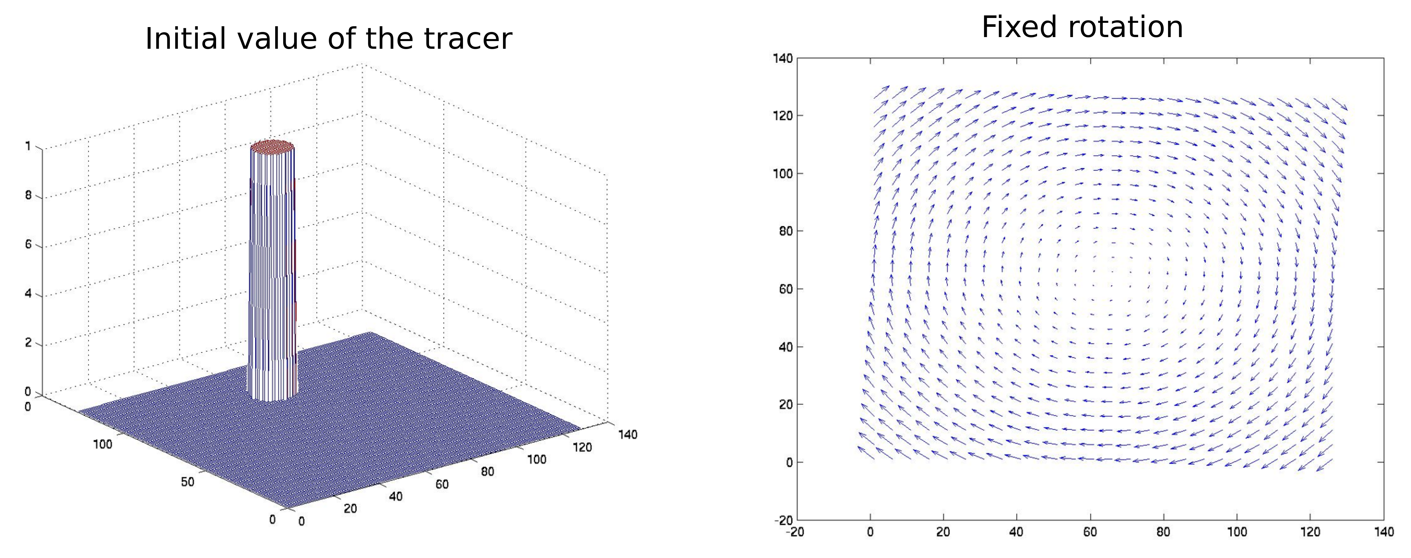
• The initial state of the problem is shown in Fig. 10: a cylindrical tracer distribution in a cylindrical velocity field. Now we propagate time until the fixed rotation has absolved one full rotation. Fig. 11 shows the resulting tracer states using different numerical propagation methods. Note how much the results differ only based on the applied scheme.

• Take home message: Discretization schemes have to be used to solve (sets of) differential equations numerically. However different schemes can yield totally different results for the same problem. Consequently the choice of the most appropriate method is crucial.

3. Parametrisation of processes on a sub-grid scale is needed as the minimal space scale is finite.

• Different ocean models work with different grids. Two examples are shown in Fig. 12. On the left you see can a tripolar grid, as used by all ORCA model configurations (Ocean model of the GEOMAR Helmholtz Centre for Oceanic Research in Kiel). North of the green line the model grid differs from a regular greographic grid with a single north pole (Courtesy: GEOMAR Helmholtz Centre Kiel). On the right the standard MPI-OM orthogonal curvilinear grid is shown.

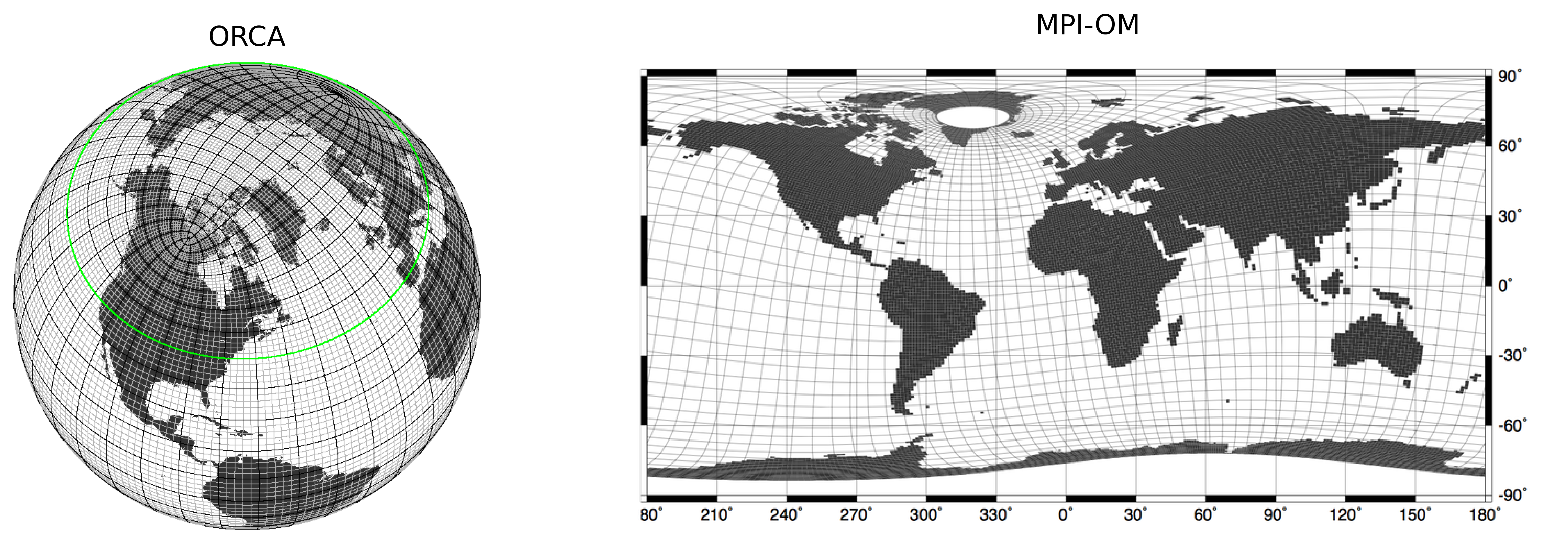
• Once again, the resolution determines the scale down to which the physical processes happening in the ocean can be included in the calculations.

• The Rossby radius of deformation is a parameter used to describe the characteristic length scale over which the effects of rotation dominate the atmospheric motion, over other forces, such as pressure gradients. It is defined as:

\[R_D = \frac{\sqrt{gh_e}}{f},\]

• \(R_D\) explains which resolutions are able to resolve eddies. The Rossby radius has to be larger than lines of grid resolution; eddie resolution is important.

• with \(g\): gravitation, \(h_e\): equivalent depth, \(f\): Coriolis parameter

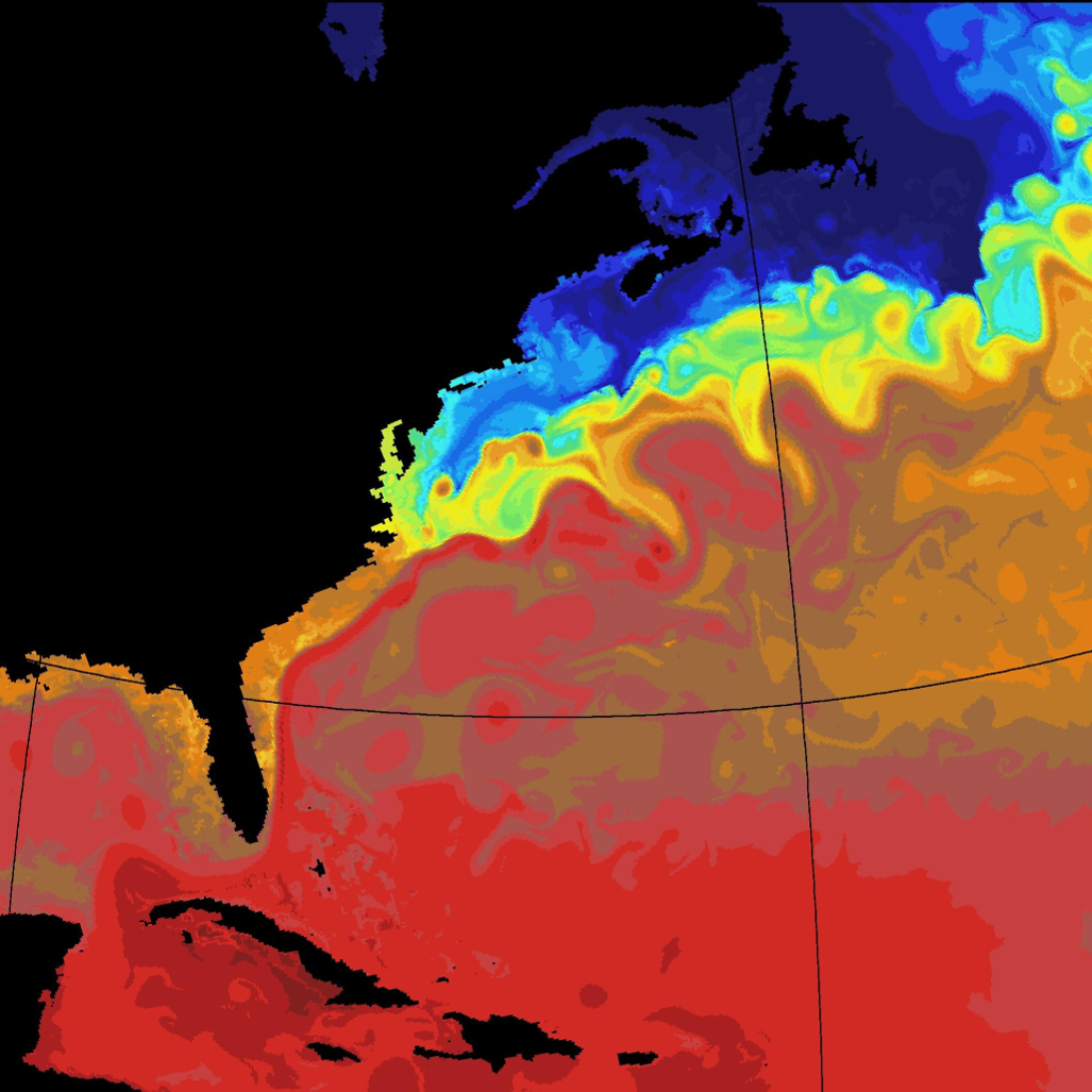
• Let’s take a look at how the Gulf Stream is resolved by a state of the art ocean model with different resolutions:

1. Gulf Stream SST

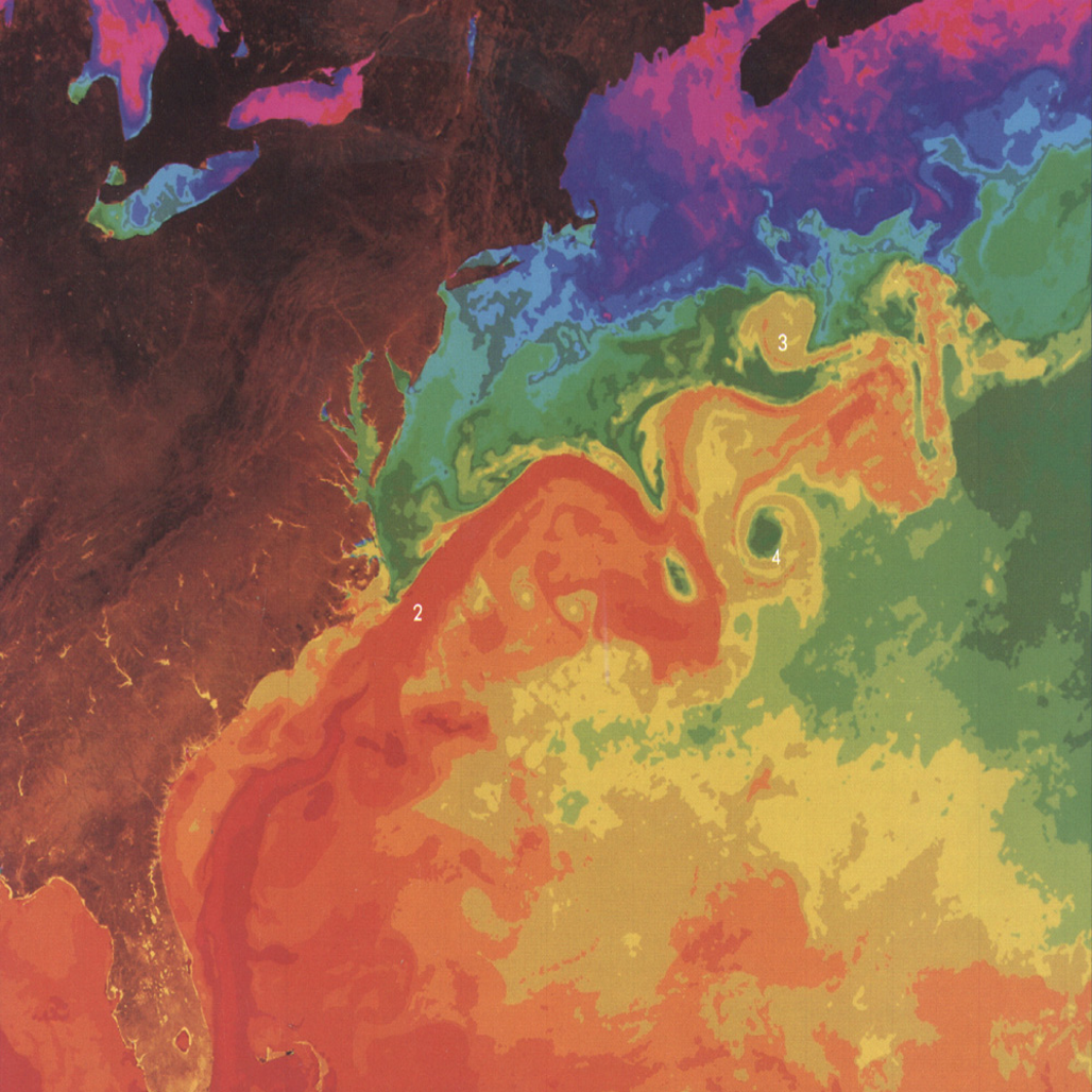
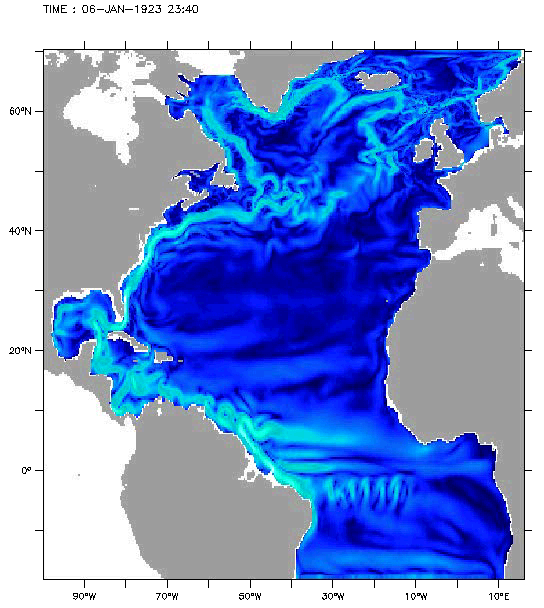
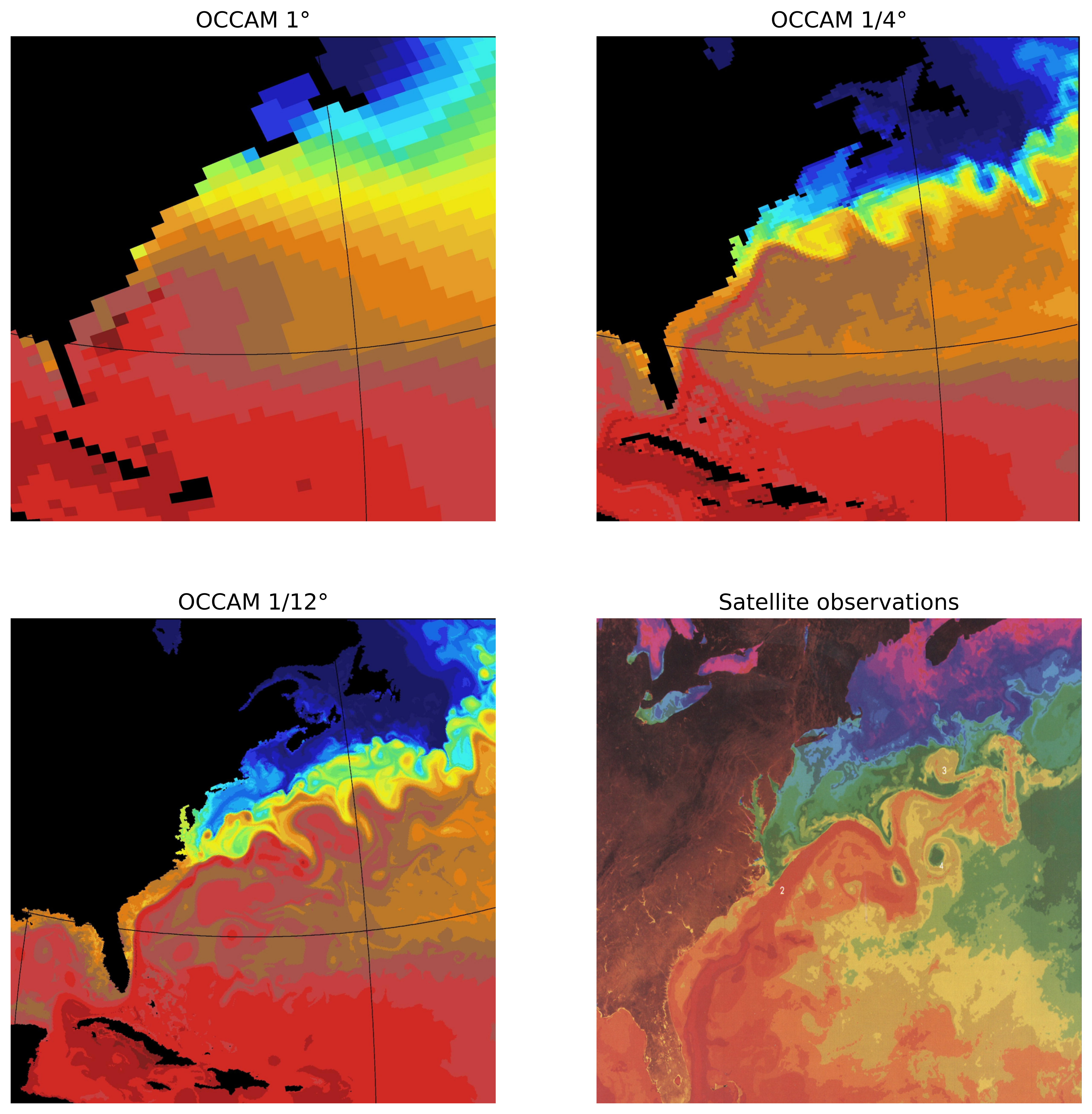
• We see that the Gulf Stream has a lot of turbulence and eddies of different sizes. The following three figures 16-18 show the SST of the same area computed by the OCCAM ocean model.

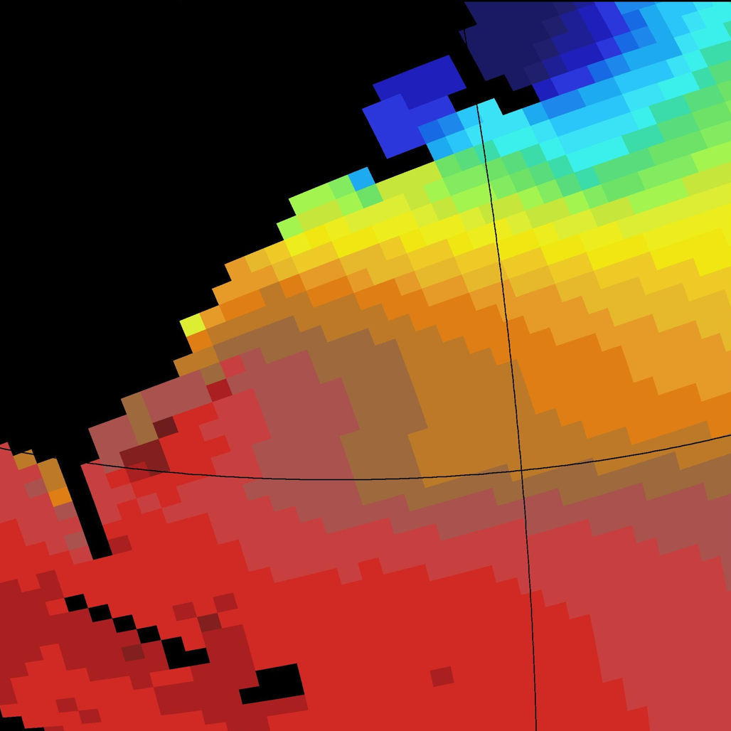
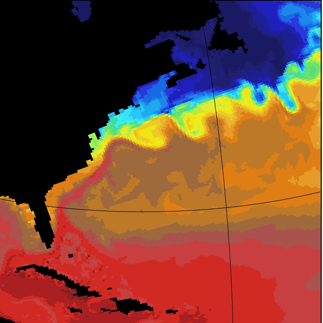
• Another plot with all four graphics in one for a better comparison in Fig. 19. One can see the difference between the 1° and the higher resolutions, which are so called “eddie-permitting”.

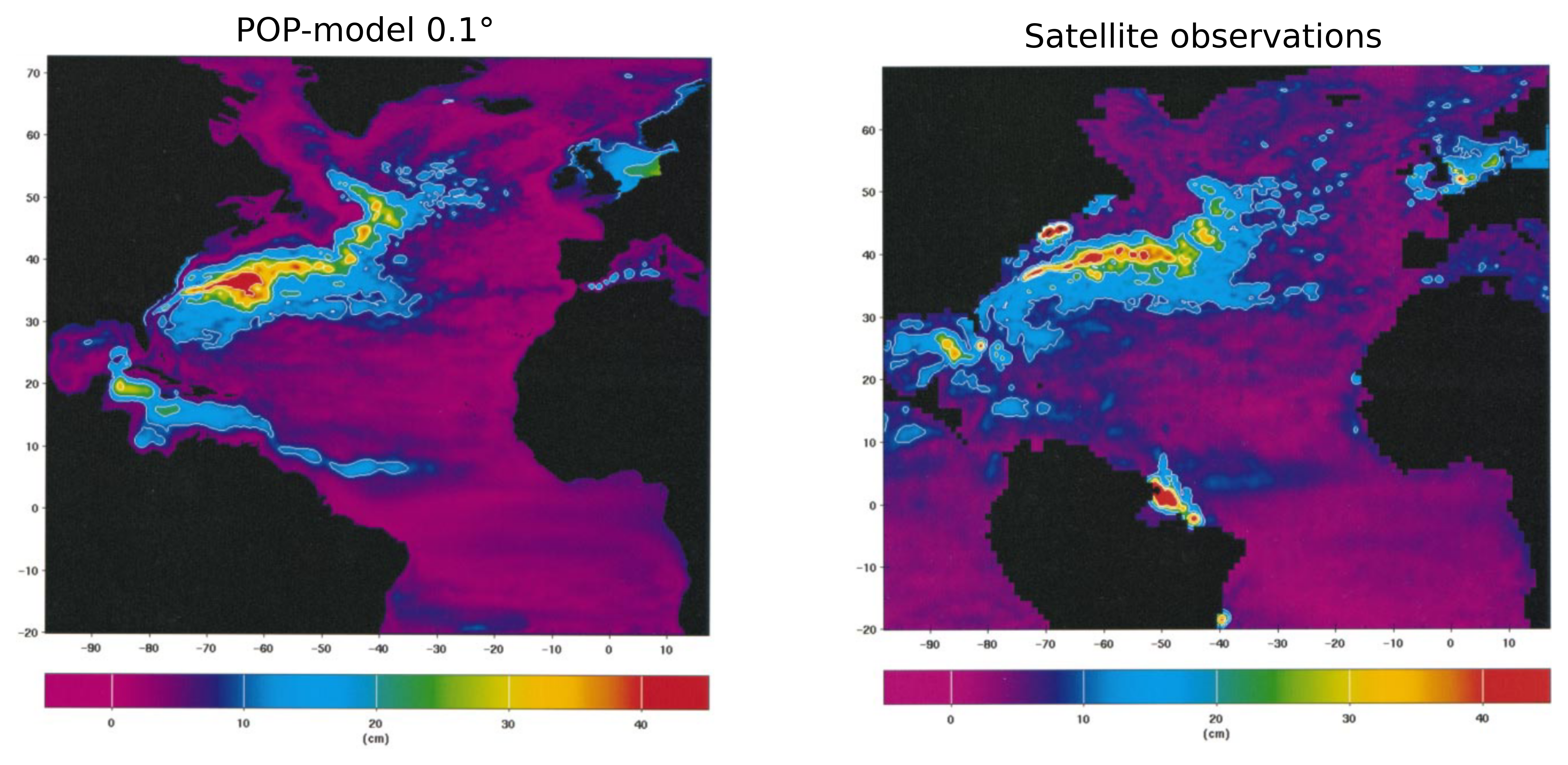
2.Sea level variability

• calculated as \(\sqrt{\bar{h'^2}}\)

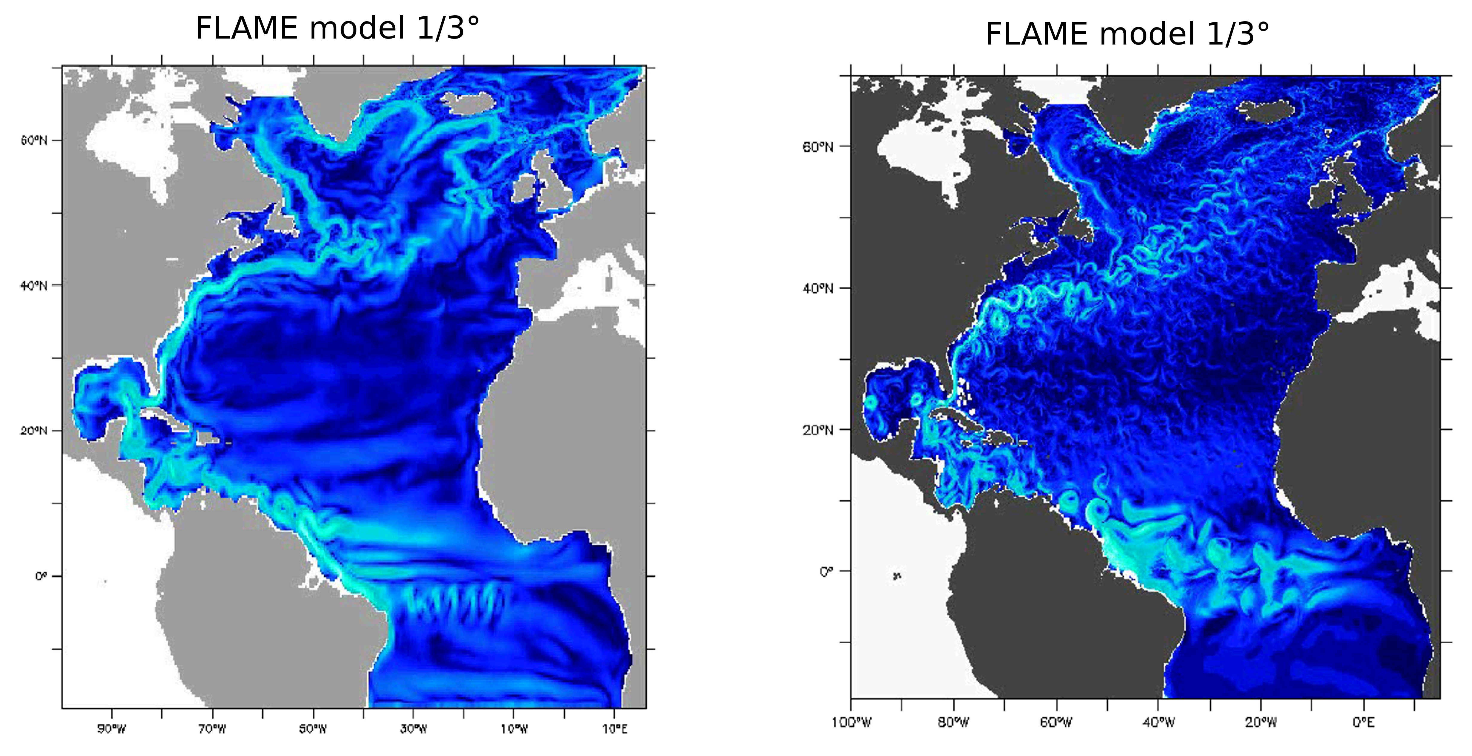
3. Velocity at 100m depth

• Fig. 21 shows the velocity at 100m depth in the ocean computed by the FLAME model with two different resolutions. Even though the resolution of 1/3° is already eddie-permitting there is a big difference to the resolution computed with a 1/12° resolution. It can be seen that the Atlantic Ocean actually consists of eddies and meanders.

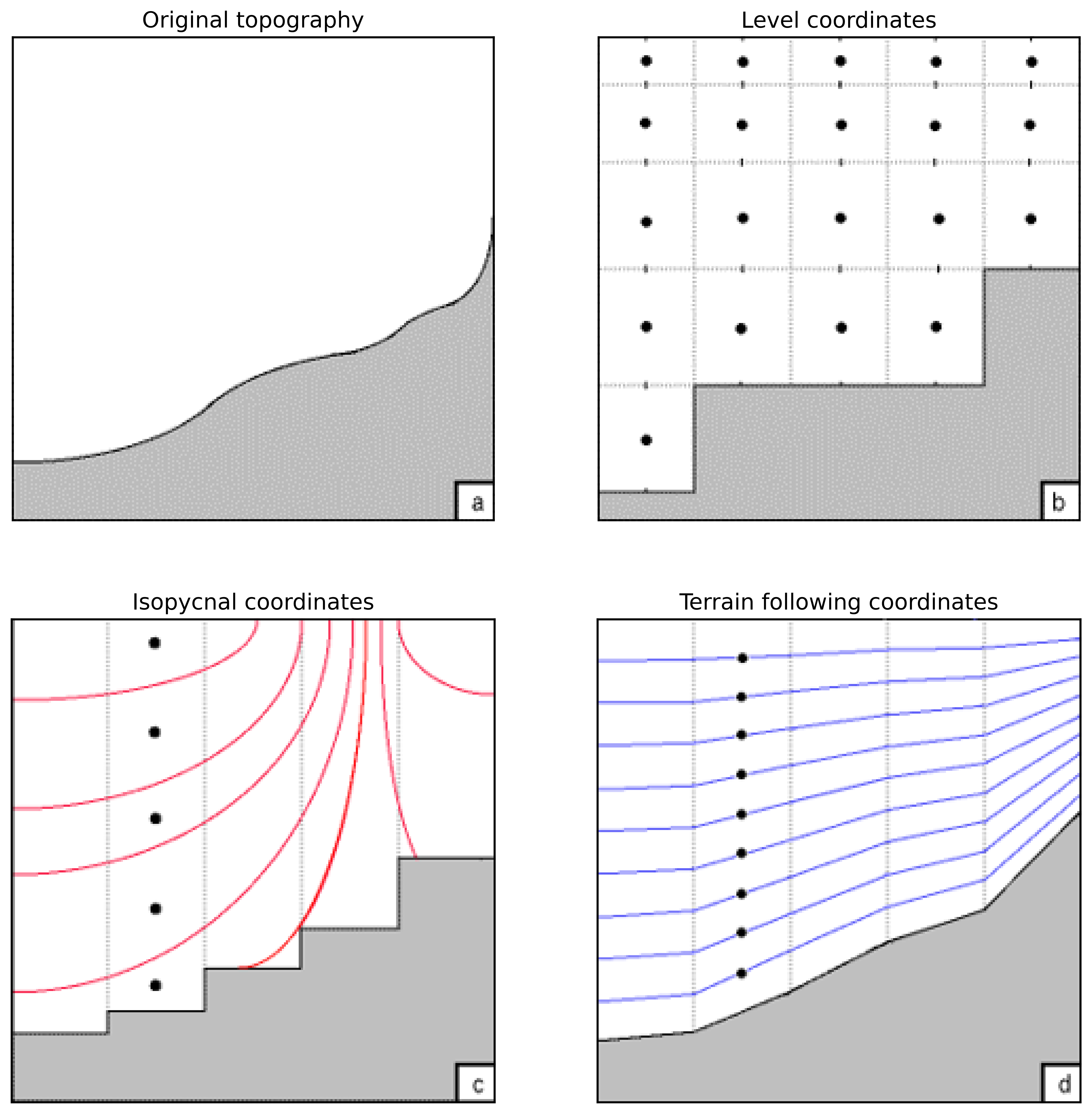
• For now we focused on the horizontal component of the coordinate system. But the vertical component is just as important! There are different solutions to the division of the vertical dimension, let’s look at three of them shown in Fig. 22.

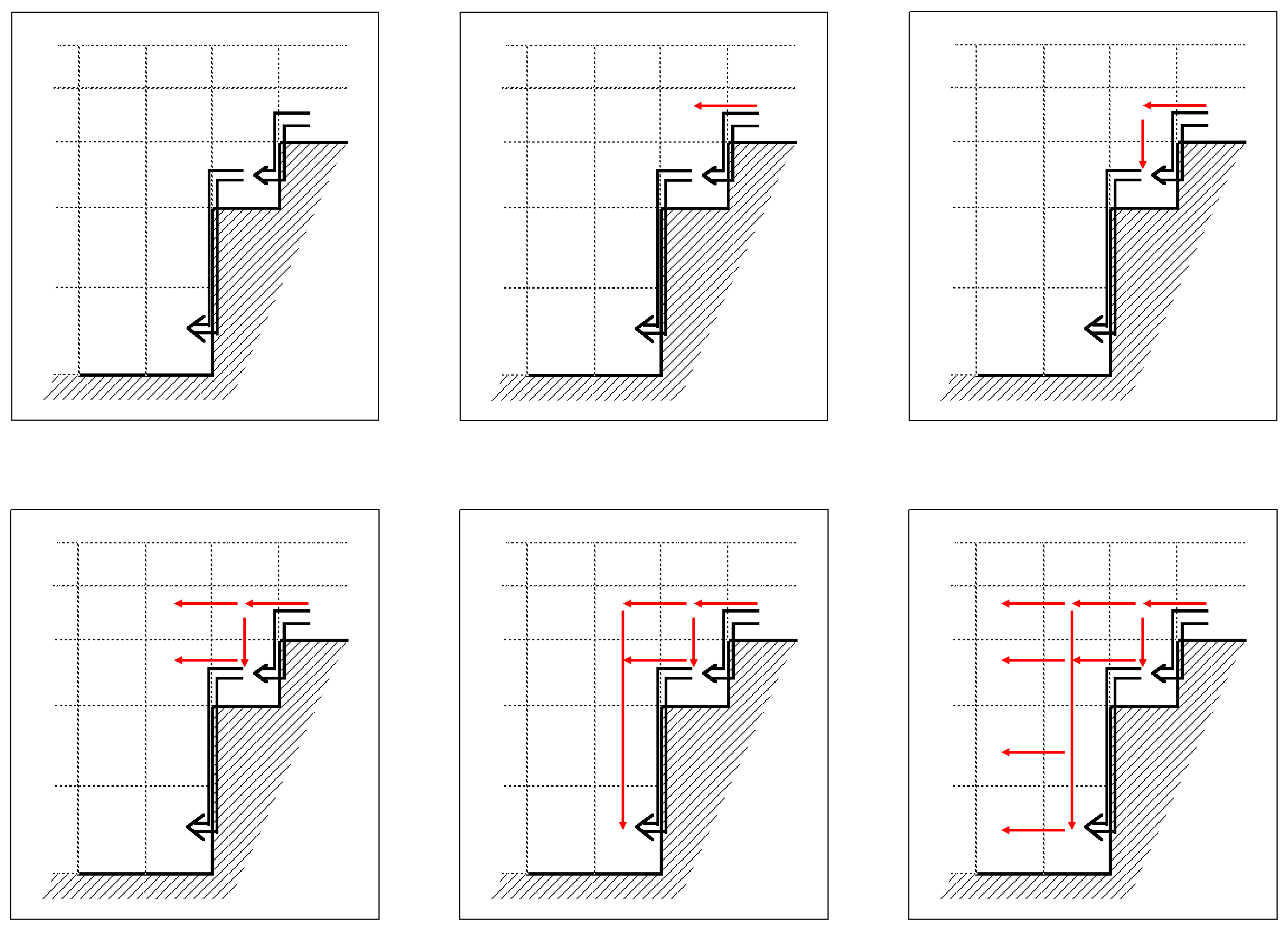
• Dense gravitational driven bottom flows pose a problem in the ocean modelling that the three prior coordinate systems solve differently well.

Evaluation of climate models

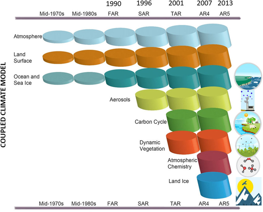
• There is a permanent thrive to improve the accuracy of climate models. They started of incorporating the atmosphere, land surface, ocean and sea ice. Over time the description of these components has improved drastically. Furthermore different components of the climate system have been added to the computations. Fig. 24 shows which climate component the computations of the IPCC Assesment Reports employ.

• Today’s GCMs reproduce large parts of the observed climate, both in terms of long term averages, variability and extreme conditions. Anyhow they certainly are far from perfect. Some weaknesses are that:

  • GCMs only represent large scale (>100km) phenomena explicitly,

  • not all GCMs include all relevant processes (e.g. carbon cycle feedback),

  • we do not fully understand how relevant processes can be described in the models

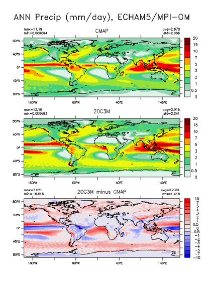
• Fig. 25 compares model results with measurements. It can be seen that the model resolves the general global patterns quite well. The problem lies in exact localisation of the patterns, a small shift in latitude between computations and measurements results in a high difference between them (see bottom plot). Better figure?

Sources of uncertainy in climate change projections

Overview

1. Emission scenario uncertainty:

   • Future behaviour of mankind is unknown

2. Modelling uncertainty:

   • Climate response to changes in atmospheric composition (GCM)

   • Modelling of ocean circulation, biogeochemistry, etc. (RCSM)

3. Uncertainty due to natural climate variability:

   • Solar activity, volcanic eruptions (external forcing)

   • Internal (=unforced) variability generated by the non-linear dynamics of the climate system

• The sources of uncertainty in model computations vary with time. Only for the first one or two decades of lead time the internal variability has a significant impact on the result. Model uncertainty (the difference between models) is largest at high latitudes and the emission scenario uncertainty grows with lead time particularly in lower latitudes. Hawkins and Sutton (2009) found that even at the end of the century the model uncertainty dominates at higher latitudes, while the emission scenario attributes for most of the explained variance at lower latitudes.

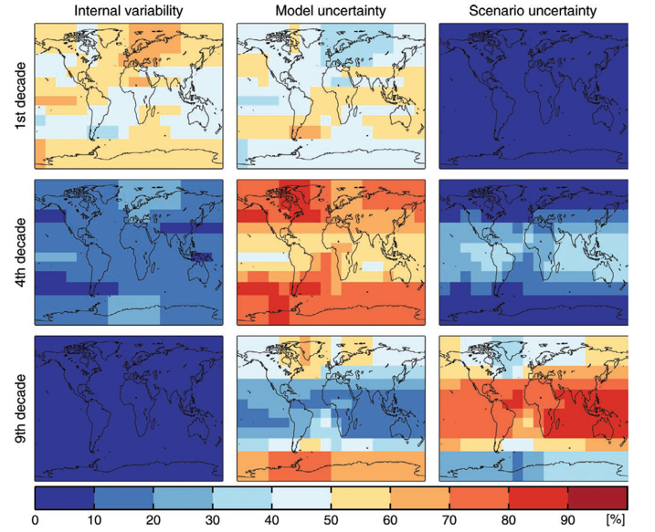
Emission scenario uncertainty

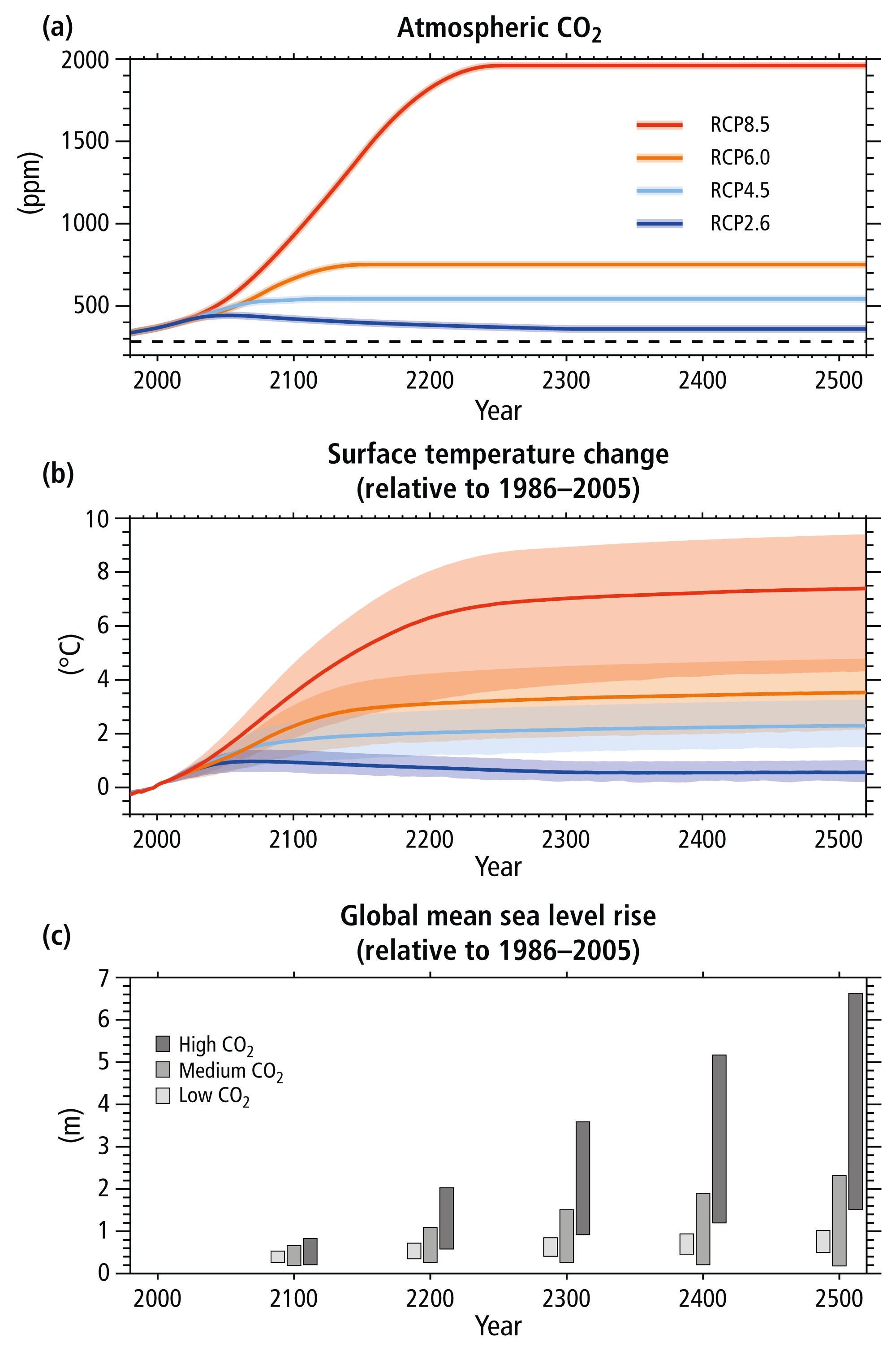
• Emission of greenhouse gases is the key component in human made climate change. In order to quantify the future emissions the IPCC has developed Representative Concentration Pathways (RCPs) representing different future emission scenarios and the caused increase in radiative forcing (the number of the RCP scenario describes the increase in radiative forcing in W/m\(^2\)). Fig. 27 shows atmospheric CO\(_2\), surface temperature change and global mean sea level rise related to different RCPs by the IPCC.

Modelling uncertainty

• Different models will compute significantly different results under the same initial conditions or ensemble runs. Fig. 28 shows different GCM projections for change trends in precipitation and temperature for Northern Sweden.

Uncertainty due to natural climate variability

Example I

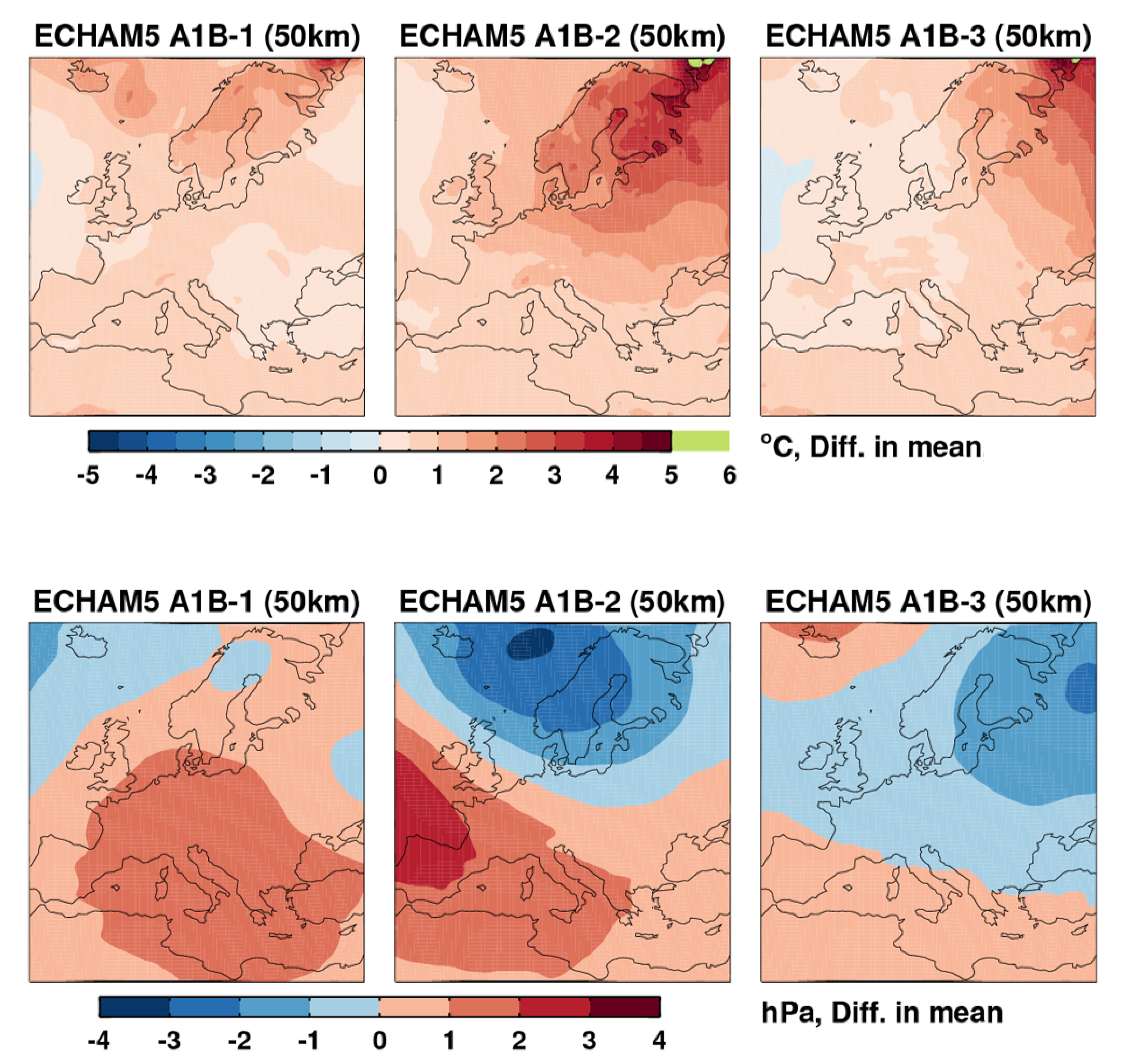
• Natural variability has a different impact on the model outpt for different variables. Fig. 29 how it affects the mean sea level spatial patterns stronger than it does for the 2m temperature.

Example II

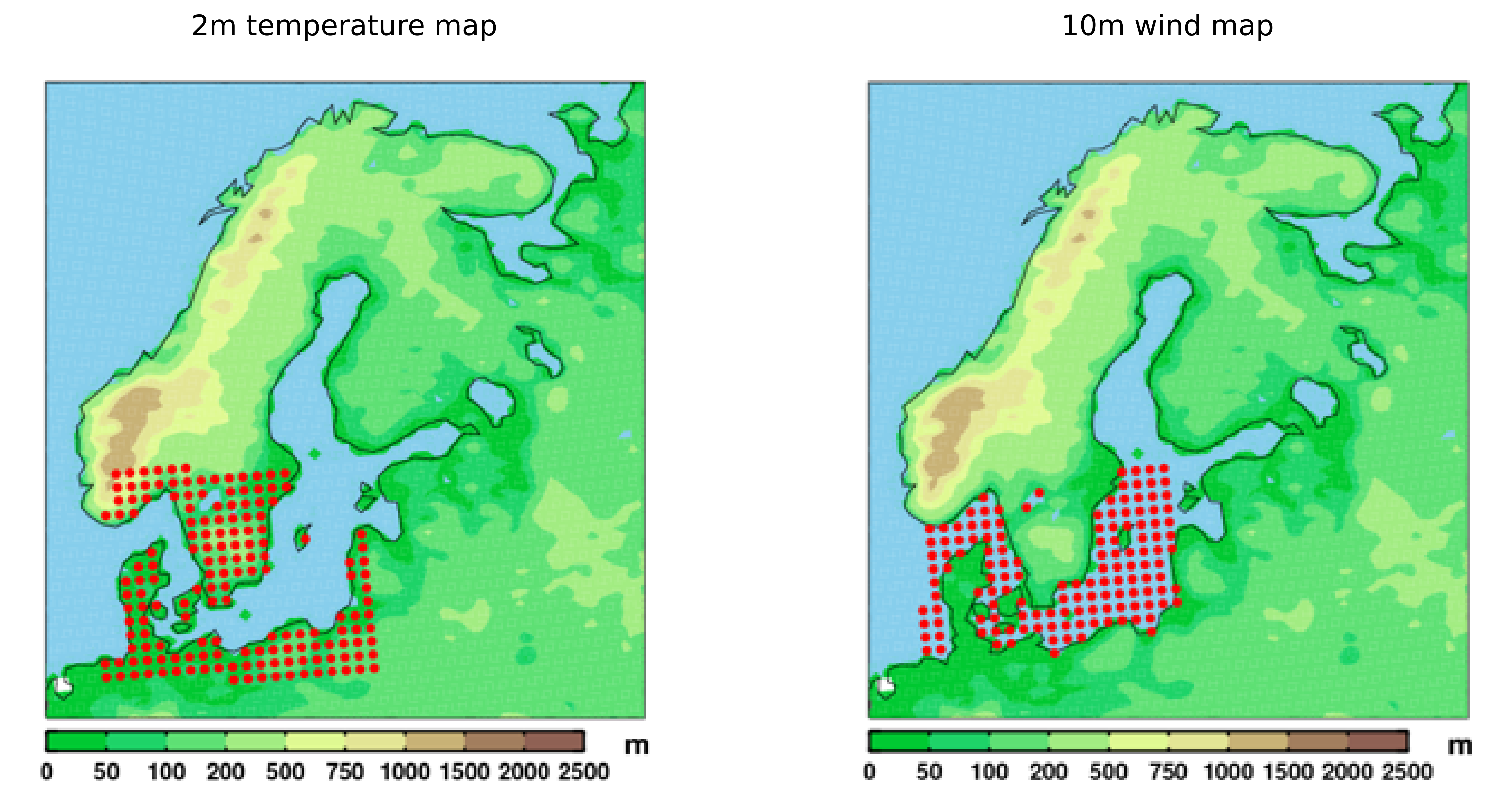
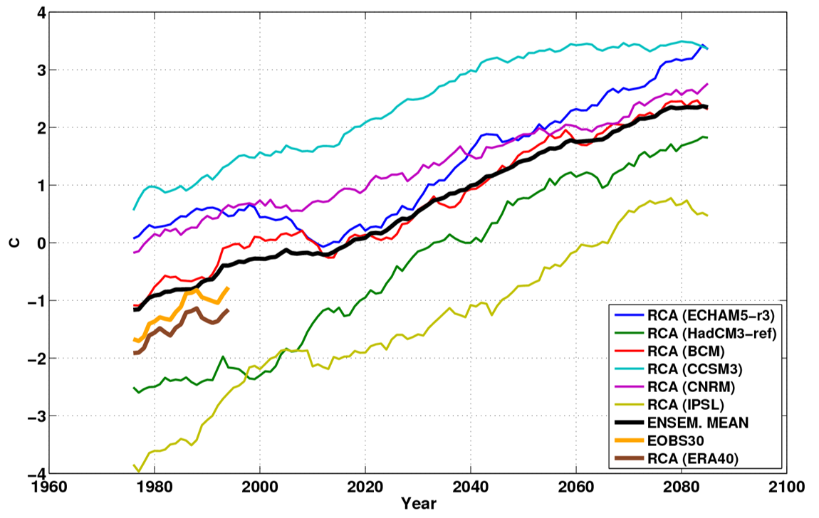
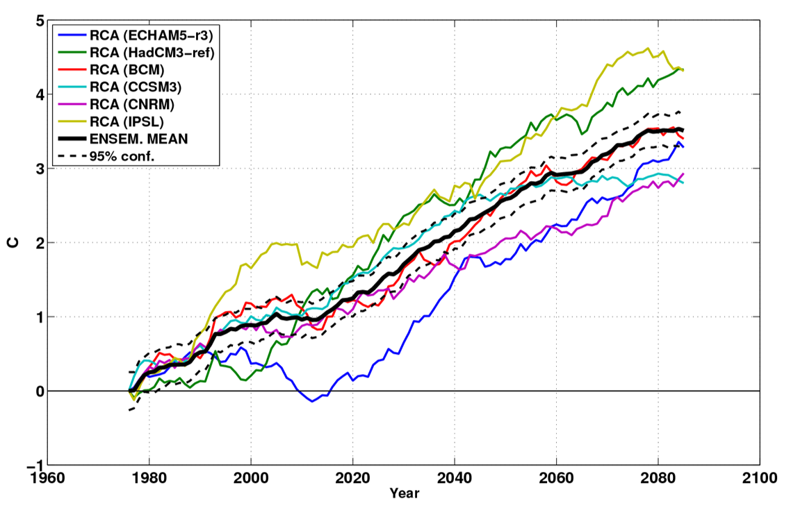
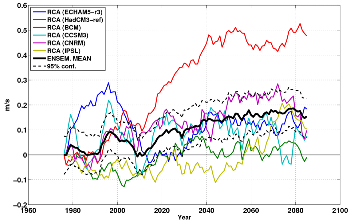
• The impact of natural climate variability on model results can also be seen comparing diifferent model results. Let’s look at one example. Different models computed the average winter 2m temperature over land and 10m wind over water for the Southern Baltic Sea region, shown in Fig. 30. Fig. 31-33 display the results using 30 year moving averages.

• All models project a gradual long term winter temperature increase, see Fig. 31. Different interpretations of the initial state cause the scalar offset between different models. This effect can be filtered out by computing the anomalies with respect to the 1961-1990 mean temperature, shown in Fig. 32. All models show a similar tendency to higher temperature with a difference among the runs of about 2K while the decadal and multi-decadal variability is fairly small.

• The winter wind projections (see Fig. 33) look totally different than the temperature projections. The ensemble mean shows a strengthening of wind over time but is strongly influenced by one model result (the RCA3(BCM)). Altogether the wind trend is highly uncertain which is caused by and showcasing the strong influence of the internal variability of the system, or in other words the natural climate variability.

Example III

• Another important, characteristic climate variable is given in precipitation. The certainty of precipitation projections varies globally. While most models agree on a positive precipitation trend close the the poles, temperature trends for lower latitudes remain fairly uncertain, as shown in Fig. 34. The precipitation trend for the Baltic Sea region is questionable for summer months (JJA), whereas most models agree on an increase in precipitation during winter months (DJF).

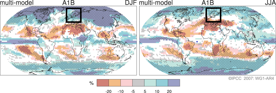
Table of Figures

Figure 1: AIR Worldwide. https://www.air-worldwide.com/publications/air-currents/2020/anatomy-of-a-climate-model/, access on 28.03.2024
Figure 2: Nichols, C. & Raghukumar, K.. Marine Environmental Characterization. Synthesis Lectures on Ocean Systems Engineering. 1. 1-103. https://doi.org/10.2200/S01006ED1V01Y202004OSE002
Figure 3: Steve Easterbrook. https://www.pinterest.de/pin/spatial-and-temporal-scales–540713498981088529/, access on 28.03.2024
Figure 4: Fig. 12.3 in Sommer, J., Chassignet, E. & Wallcraft, A. (2018). Ocean circulation modeling for operational oceanography:current status and future challenges.
Figure 5: Figure 1-14 in IPCC AR5, https://www.ipcc.ch/report/ar5/wg1/introduction/gmt-v4-3-1-document-from-psxyz/
Figure 6: AIR Worldwide. https://www.air-worldwide.com/publications/air-currents/2020/anatomy-of-a-climate-model/, access on 28.03.2024
Figure 7 and 8: Source: J. Dengg as of PP. Any more info? Could find’t the figures on google
Figure 9: Figure 5 in Dietze, H., Löptien, U. & Getzlaff, J.: MOMSO 1.0 – an eddying Southern Ocean model configuration with fairly equilibrated natural carbon, Geosci. Model Dev., 13, 71–97, https://doi.org/10.5194/gmd-13-71-2020, 2020.
Figure 10 left: Figure 2.1 top left in Master thesis of Strömgren, T. Implementation of a Flux Corrected Transport scheme in the Rossby Centre Ocean model. Swedish Meteorological and Hydrological Institute (2005).
Figure 10 right: Figure 2.1 top right in Master thesis of Strömgren, T. Implementation of a Flux Corrected Transport scheme in the Rossby Centre Ocean model. Swedish Meteorological and Hydrological Institute (2005).
Figure 11 left: Figure 2.1 bottom right in Master thesis of Strömgren, T. Implementation of a Flux Corrected Transport scheme in the Rossby Centre Ocean model. Swedish Meteorological and Hydrological Institute (2005).
Figure 11 middle: Figure 2.1 bottom left in Master thesis of Strömgren, T. Implementation of a Flux Corrected Transport scheme in the Rossby Centre Ocean model. Swedish Meteorological and Hydrological Institute (2005).
Figure 11 right: Figure 3.5 bottom right in Master thesis of Strömgren, T. Implementation of a Flux Corrected Transport scheme in the Rossby Centre Ocean model. Swedish Meteorological and Hydrological Institute (2005).
Figure 12 left: GEOMAR Helmholtz Centre for Ocean Research Kiel, https://www.geomar.de/fb1-od/ozean-modelle-hpc, access on 02.04.2024
Figure 12 right: Fig. 1 in Jungclaus, J. & Bonzet, M & Haak, Helmuth & Keenlyside, Noel & Luo, Jing-Jia & Latif, M. & Marotzke, J. & Mikolajewicz, U. & Reockner, E. (2006). Ocean circulation and tropical variability in the coupled model ECHAM5/MPI-OM. J. Climate. https://doi.org/10.1175/JCLI3827.1.
Figure 13: Steve Easterbrook. https://www.pinterest.de/pin/spatial-and-temporal-scales–540713498981088529/, access on 28.03.2024
Figure 14: Fig. 1 in Smith, R. D., M. E. Maltrud, F. O. Bryan, and M. W. Hecht, 2000: Numerical Simulation of the North Atlantic Ocean at 1/10°. J. Phys. Oceanogr., 30, 1532–1561, https://doi.org/10.1175/1520-0485(2000)030<1532:NSOTNA>2.0.CO;2.
Figure 15-18: A. Coward as of PP. Any more info? Could find’t the figures on google
Figure 20: left: Fig. 17(B) in Smith, R. D., M. E. Maltrud, F. O. Bryan, and M. W. Hecht, 2000: Numerical Simulation of the North Atlantic Ocean at 1/10°. J. Phys. Oceanogr., 30, 1532–1561, https://doi.org/10.1175/1520-0485(2000)030<1532:NSOTNA>2.0.CO;2.
Figure 20: right: Fig. 17(C) in Smith, R. D., M. E. Maltrud, F. O. Bryan, and M. W. Hecht, 2000: Numerical Simulation of the North Atlantic Ocean at 1/10°. J. Phys. Oceanogr., 30, 1532–1561, https://doi.org/10.1175/1520-0485(2000)030<1532:NSOTNA>2.0.CO;2.
Figure 21: J. Dengg as of PP. Any more info? Could find’t the figures on google
Figure 22: http://www.ifm.uni-kiel.de/fb/fb1/tm/research/dynamo/dyn_m.html as of PP. Any more info? Link is no longer valid
Figure 24: Figure 2 in Ambrizzi, Tércio & Reboita, Michelle & Rocha, Rosmeri & Llopart, Marta. (2018). The state-of-the-art and fundamental aspects of regional climate modeling in South America. Annals of the New York Academy of Sciences. 1436. https://doi.org/10.1111/nyas.13932.
Figure 26: Figure 6 in Hawkins, E., and R. Sutton, 2009: The Potential to Narrow Uncertainty in Regional Climate Predictions. Bull. Amer. Meteor. Soc., 90, 1095–1108, https://doi.org/10.1175/2009BAMS2607.1.
Figure 27: Figure 2.8 in IPCC, 2014: Climate Change 2014: Synthesis Report. Contribution of Working Groups I, II and III to the Fifth Assessment Report of the Intergovernmental Panel of Climate Change [Core Writing Team, R.K. Pachauri and L.A. Meyer (eds.)]. IPCC, Geneva, Switzerland, 151pp. in IPCC AR5 Synthesis Report
Figure 30 - Figure 33: Courtesy of G. Nikolin, SMHI
Figure 34: Figure 3.3 in IPCC, 2007: Climate Change 2007: Synthesis Report. Contribution of Working Groups I, II and III to the Fourth Assessment Report of the Intergovernmental Panel on Climate Change [Core Writing Team, Pachauri, R.K and Reisinger, A. (eds.)]. IPCC, Geneva, Switzerland, 104 pp.