Buoyancy-driven circulation

Buoyancy-driven circulation#

What makes the ocean circulate in the way it does?#

Some numbers around the ocean:

Ocean covers \(\mathrm{70\%}\) of Earth’s surface
\(\mathrm{57\%}\) of the oceans are in the Southern Hemisphere (consists of \(\mathrm{80\%}\) ocean)
Average depth of \(\mathrm{3.7km}\)
Volume of the world ocean is \(\mathrm{1.3*10^{18}m^3}\) (density of sea water around \(\mathrm{1.03*10^{3}\frac{kg}{m^3}}\)
Total mass of the ocean: \(\mathrm{1.4*10^{21}kg}\), compared to the mass of the atmosphere: \(\mathrm{5*10^{18}kg}\)
Specific heat of sea water \(\mathrm{4.180\frac{J}{kgK}}\) resulting in an overall heat capacity of the ocean which is 1000 that of the atmosphere -> ocean’s moderating effect on climate

Transports in the ocean:

\(\mathrm{1Sv = 10^6 \frac{m^3}{s}}\)
Antarctic Circumpolar Current (ACC) transporting \(\mathrm{120Sv}\), in some places up to \(\mathrm{150Sv}\)
Gulf Stream carries \(\mathrm{30Sv}\) off the coast of Florida, and \(\mathrm{150Sv}\) at Cape Hatteras in North Carolina
Amazon river carries \(\mathrm{0.2Sv}\)
All the world’s rivers into the ocean: \(\mathrm{1Sv}\)
Westerly winds in the atmosphere carry up to \(\mathrm{500Sv}\)

main drivers of ocean circulation are surface winds & buoyancy effects:
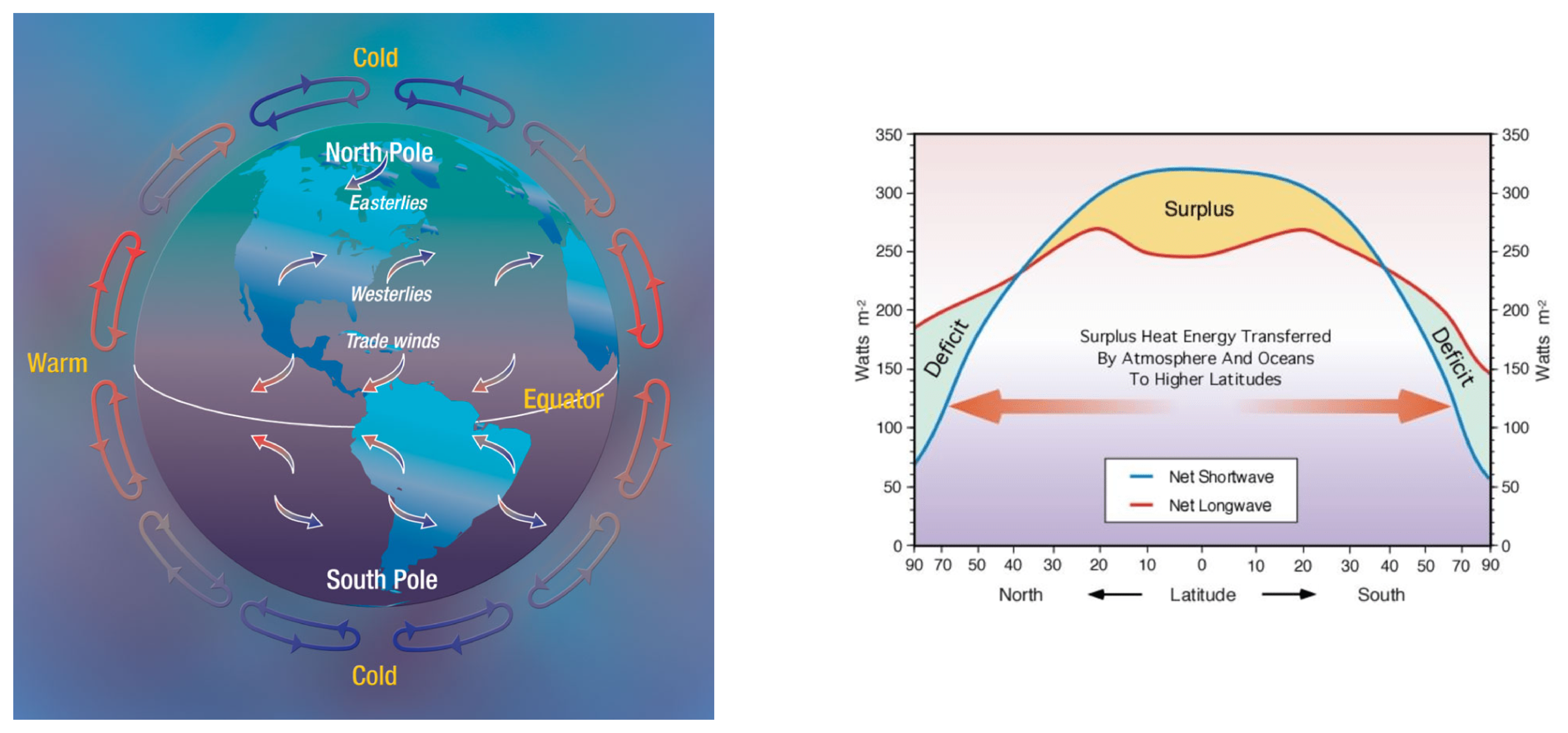
1. zonal winds force gyers. gyer rotation directions indicate the impact of the surface winds as they agree with the zonal wind directions -> compare Fig. 1 (left) with Fig. 2 (left). wind also plays a role for the interhemispheric meridional overturning ciculation (MOC) through upwelling: strong westerly winds in the Antarctic Circumpolar Current (ACC) can draw water up from the deep and induce interhemispheric circulation, which is particularly strong for the Atlantic.
2. buoyancy effects include temperature and salinity gradients. mixing brings solar heat down to the abyss at low latitudes, which may then rise through the thermocline, maintaining a circulation of sinking at high latitudes and rising at low latitudes, enabling a MOC to be maintained. salinity forcing is mainly of oppsite direction since salinity decreases with altitude due to decreasing evaporation and increasing freshwater input through precipitation and river runoff. in our current climate state the temperature effects are dominant. Courtesy: G. Vallis

As a simplification the global conveyor belt can be interpreted as the ACC with MOC branches reaching into the three main oceanic basins of the Atalntic, Pacific and Indian Ocean (see https://upload.wikimedia.org/wikipedia/commons/a/ab/Thermohaline_circulation.svg for a nice animation).
The ACC is driven by strong westerlies all around the Antarctic continent (see the panel on the left side of Fig. 1).

Driving mechanisms: If there would be no mixing (turbulent diffusion generated by mechanical forcing - wind and tides) and no upwelling around Antarctica (due to Ekman transport) the ocean would be in the “cold death” steady state. In todays climate the MOC is thermally driven, rather han salt driven, as already previously mentioned. But the salinity explains hte difference between the MOC of the Atlantic (NA is saltier) and the Pacfific.
Time scales: Currents in the abyssal ocean have chacteristic speeds of \(\mathrm{1\frac{mm}{s}}\), so that it takes 300 years for a parcel from a high latitude source to move to the equator. If the surface conditions change, it will take several hundret years for the deep ocean to re-equilibrate. Courtesy: G. Vallis

The Atlantic Meridional Overturning Circulation (AMOC)#

Paleoclimate temperature series for Greenland:

Temperature series from the last ice age indicate strong and sudden changes, as seen for Greenland in Fig. 6 and 7. The most recent example is the Younger Dryas indicated in Fig. 7. The leading hypothesis to explain this massive drop in temperature reasons it with the AMOC being interrupted by a large influx of freshwater -> the AMOC can have large impact on Northern Hemisphere climate!
The AMOC can adopt different states depending on the oceanic ice cover, shown in Fig. 8. The bottom Earth (left) and circulation (right) depict a climate state as currently prevailing, with little ice cover. The AMOC is strong and transports warm surface water polewards, where the water releases its heat and forms deep water. The top Earth (left) and circulation sketch (right) show the AMOC for a largely ice-covered Northern Hemisphere. The circulation is weaker and reversed in its direction transporting water southward. In the middle an in between climate state is shown, you can see how the surface flow cannot propagate as far North anymore because the ocean is frozen there.

Now the impulse of a climate physicist is to ask: How can I model the AMOC? Henry Stommel asked himself the same question and in 1961 he came up with his two-box model as an answer.

Stommel’s two-box model#

Simplifying the AMOC: splitting the North Atlantic into two boxes by latitude, the subtropical box and the polar box. The exchange between the boxes is density and thus temperature and salinity driven.

There is a strong meridional temperature gradient in the Atlantic Ocean, so the two boxes mark areas with distinctly different temperature profiles, as shown in Fig. 10. Intuitively the polar box in higher latitudes has a lower temprature than the subtropical box.

Lower latitudes accomodate higher salinities than higher latitudes in the North Atlantic, as shown in Fig. 11. This is due to a difference in evaporation, which is higher for the subtropical box, and a difference in freshwater supply, which is higher for the polar box where the ocean experiences more precipitation and river runoff.

The model navigates the dynamics between a temperature and a salinity driven regime. They have opposite direction as shown in Fig. 14. We know that in our current climate state the temperature driven circulation dominates.

The model includes temperature exchange with the atmosphere for the subtropical box and salinity exchange for the polar box. The salinity exchange yields from freshwater influx, which decreases the oceanic salinity. The two boxes are connected and exchange water through cannels on top and bottom in a water cycle. Due to continuity the net mass flow has to be zero, so for each gramm of water transported poleward on the surface one gramm of water flows back South at the bottom.

Let’s take a look at the governing equations of the system. Fig. 15 shows temperature \(\mathrm{T}\), salinity \(\mathrm{S}\) and volume \(\mathrm{V}\) of the subtropical (index \(\mathrm{s}\)) and the polar (index \(\mathrm{p}\)) box. Index \(\mathrm{a}\) indicates the atmosphere which the two boxes are in exchange with. The flow is driven by a difference in density between the two boxes. The flow \(\Psi\) is positive if the surface flow is northwards.

(19)#\[\Psi = \alpha (\rho_p - \rho_s).\]

We assume the density of both boxes to be a linear function of temperature and salinity respectively.

(20)#\[\rho = \rho_0(1-\beta_TT + \beta_SS)\]

These assumptions yield the governing equations for temperature and salinity of the subtropical and the polar box \(T_s\), \(T_p\), \(S_s\) and \(S_p\) with coupling parameters \(\lambda_T\) and \(\lambda_S\) between atmosphere and ocean:

(21)#\[\begin{split}\begin{align*} \frac{dT_s}{dt} &= |\Psi|(T_p-T_s) + \lambda_T(T_s^a-T_s)\\ \frac{dT_p}{dt} &= |\Psi|(T_s-T_p) + \lambda_T(T_p^a-T_p)\\ \frac{dS_s}{dt} &= |\Psi|(S_p-S_s) + \lambda_S(S_s^a-S_s)\\ \frac{dS_p}{dt} &= |\Psi|(S_s-S_p) + \lambda_S(S_p^a-S_p) \end{align*}\end{split}\]

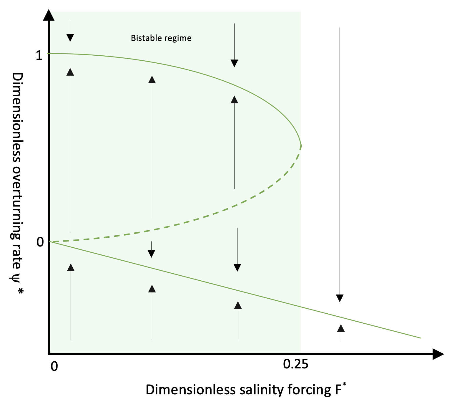
Taking (19) and (32) into account the system of differential equations (21) can be solved. Under certain circumstances we can get a solution with three branches as shown in Fig. 16 - each branch represents are possible equilibrium. A positive dimensionless overturning rate means polewards surface flow, and a negative rate means surface flow towards the equator.
At the current state of the climate system the AMOC state lays on the upper solid branch. A strong increase in salinity forcing (\(F^* > 0.25\)) would cause the system to fall onto the lower branch which corresponds to a flippening of the circulation. The dashed line represents an unstable equilibrium: a small perturbation in the salinity forcing will get amplified and the system navigates to one of the two stable equilibria.
This is more than just a thought experiment, because the AMOC is one of the global tipping points of Earth’s climate system. Due to climate change the meridional temperature gradient along the Atlantic Ocean decreases. Furthermore freshwater influxes into the North Atlantic due to melting glacier ice masses are effectively increasing the meridional salinity gradient. Both processes weaken the AMOC until… at some point we could eventually reach its tipping point.

Several climate models have computed the effects of an AMOC shutdown. Fig. 17 shows one result. A shutdown would lead to a drastical cooling of the whole Northern Hemisphere and especially of the Northern Atlantic - which is intuitive since the transport of warm surface waters to the North would stop.

Courtesy: D. Dommenget

Table of figures#

Figure 1: Left: Figure 2.3 in Vallis, Geoffrey K.. Climate and the Oceans. Princeton University Press, 2012. Right: Figure ??? in Vallis, Geoffrey K.. Climate and the Oceans. Princeton University Press, 2012.
Figure 2: Left: Copyright UCAR Center for Science Education. https://scied.ucar.edu/learning-zone/how-weather-works/global-air-atmospheric-circulation. Right: Copyright M. Pidwirny, 2006. www.physicalgeography.net.
Figure 3: Figure ??? in Vallis, Geoffrey K.. Climate and the Oceans. Princeton University Press, 2012.
Figure 4: Figure 4.6 in Vallis, Geoffrey K.. Climate and the Oceans. Princeton University Press, 2012.
Figure 5: Figure 4.8 in Vallis, Geoffrey K.. Climate and the Oceans. Princeton University Press, 2012.
Figure 6: Figure 6.111 in the lecture notes of Dietmar Dommenget: An Introduction to Climate Dynamics, https://users.monash.edu.au/~dietmard/teaching/dommenget.climate.dynamics.lecture.notes.pdf
Figure 7: Figure 6.112 in the lecture notes of Dietmar Dommenget: An Introduction to Climate Dynamics, https://users.monash.edu.au/~dietmard/teaching/dommenget.climate.dynamics.lecture.notes.pdf
Figure 8: Figure 6.113 in the lecture notes of Dietmar Dommenget: An Introduction to Climate Dynamics, https://users.monash.edu.au/~dietmard/teaching/dommenget.climate.dynamics.lecture.notes.pdf
Figure 9: Figure 6.115 in the lecture notes of Dietmar Dommenget: An Introduction to Climate Dynamics, https://users.monash.edu.au/~dietmard/teaching/dommenget.climate.dynamics.lecture.notes.pdf
Figure 10: Figure 6.116 in the lecture notes of Dietmar Dommenget: An Introduction to Climate Dynamics, https://users.monash.edu.au/~dietmard/teaching/dommenget.climate.dynamics.lecture.notes.pdf
Figure 11: Figure 6.117 in the lecture notes of Dietmar Dommenget: An Introduction to Climate Dynamics, https://users.monash.edu.au/~dietmard/teaching/dommenget.climate.dynamics.lecture.notes.pdf
Figure 12: Figure 6.118 in the lecture notes of Dietmar Dommenget: An Introduction to Climate Dynamics, https://users.monash.edu.au/~dietmard/teaching/dommenget.climate.dynamics.lecture.notes.pdf
Figure 13: Figure 6.119 in the lecture notes of Dietmar Dommenget: An Introduction to Climate Dynamics, https://users.monash.edu.au/~dietmard/teaching/dommenget.climate.dynamics.lecture.notes.pdf
Figure 14: Figure 6.120 in the lecture notes of Dietmar Dommenget: An Introduction to Climate Dynamics, https://users.monash.edu.au/~dietmard/teaching/dommenget.climate.dynamics.lecture.notes.pdf
Figure 16: By Deniseruijsch - Own work, CC BY-SA 4.0, https://commons.wikimedia.org/w/index.php?curid=105284780
Figure 17: Figure 6.128 in the lecture notes of Dietmar Dommenget: An Introduction to Climate Dynamics, https://users.monash.edu.au/~dietmard/teaching/dommenget.climate.dynamics.lecture.notes.pdf