Red noise#
Simple red noise null hypothesis
Hasselmann (as explained by Dommenget and Latif, 2000)#
Hasselmann (1976) attempts to explain the mechanism of natural climate variabilty by dividing the climate system into a fast system and a slow system. The fast system could be the atmosphere, represented as white noise. The slower component is the ocean and is explained by the integration of white noise (AR-1). In this picture the ocean is merely a passive part of the climate system, which amplifies long-term variability, due to its large heat capacity, but dynamical processes in the ocean are not considered.
The resulting stochastic model of the SST variability is described by an autoregressive process of the first order, which is the simplest statistical model that can be applied to a stationary process. The stochastic climate model by Hasselmann is tehrefore often chosen as the null hypothesis of SST variability.
Slab ocean-atmosphere models can be regarded as a numerical realization of the null hypothesis (AR(1)-process) of Hasselmann’s stochastic climate model.
The null hypothesis of SST variability in the midlatitudes, described by Hasselmann’s stochastic climate model, assumes that the SST variability is well described by the integration of the atmospheric heat flux with the heat capacity of the ocean’s mixed layer.
\(\frac{d SST}{dT} = \frac{1}{C_p \rho_w d_{mix}}* F + \Delta T_c\)
\(C_p\) = specifc heat of sea water
\(\rho_w\) = density of sea water
\(d_{mix}\) = depth of mixed layer
\(F\) = net atmospheric heat flux
\(\Delta T_c\) = climatology temperature correction
The only free parameter in this eqaution is the mixed layer depth, which was chosen to be 50 meters for all points. This value is roughly the global mean vlaue for the mixed layer depth as was determinded from the observations by Levitus (1982).
Redness of the SST anomalies#
The standard deviation of the SST anoamlies do not aloine describe the large-scale character of the SST varaiblity. An important feature of the SSt variability is the increase of the variance in the SST power spectra with period, which is the so called redness of the spectra. If the SST anomalies follow an AR(1)-process than the redness can be estimated by the lag-1 correlation.
\(C(\omega) = \frac{\sigma^2}{(1-\alpha)^2+\omega^2}\)
\(\sigma\) = standard deviation
\(\omega\) = frequency
\(\alpha\) = lag-1 correlation based on monthly mean time series
The increase of \(C(\omega)\) is only a function of \(\alpha\), hence the redness \(Q_{red}\) can be defined as
\(Q_{red}\) = \(\frac{1}{(1-\alpha)^2}\)
Conclusions#
fully coupled models are signifcantly different in terms of large-scale features of the SST variability than slab ocean models
only slab ocean models can be regarded as an AR(1) process
The diference between the AR(1)-process and the SST spectra in the simulations with fully dynamical ocean models is characterized by a slower increase of the SST variance from the shorter time periods to the longer time periods, which leads to increased variance of the SST on the seasonal and the decadal timescale relative to the fitted AR(1)-process. AMO and AMOC.
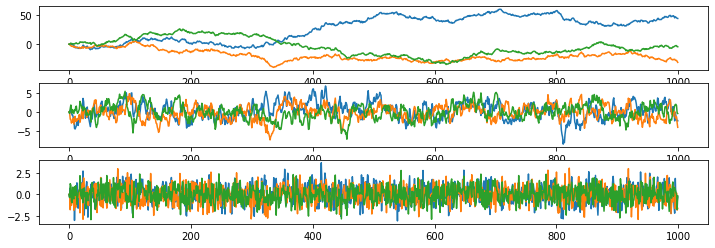
Simple red noise null hypothesis#
#hide_input
import numpy as np
import matplotlib.pyplot as plt
c1 = 1
c2 = 0.86
c3 = 0.01

f, ax = plt.subplots(3, figsize = (12,4))
ax = ax.ravel()

for realisation in range(0,3):

    white_noise_sequence = np.random.normal(0, 1, 1000)
    red_noise_sequence1 = np.zeros((len(white_noise_sequence)))
    red_noise_sequence2 = np.zeros((len(white_noise_sequence)))
    red_noise_sequence3 = np.zeros((len(white_noise_sequence)))

    for i in range(1, len(white_noise_sequence)):

        red_noise_sequence1[i] =  c1 * red_noise_sequence1[i-1] + white_noise_sequence[i]
        red_noise_sequence2[i] =  c2 * red_noise_sequence2[i-1] + white_noise_sequence[i]
        red_noise_sequence3[i] =  c3 * red_noise_sequence3[i-1] + white_noise_sequence[i]

    ax[0].plot(red_noise_sequence1)
    ax[1].plot(red_noise_sequence2)
    ax[2].plot(red_noise_sequence3)