Lecture 6, Heat transports

Two-dimensional advection-diffusion of heat

import xarray as xr
import numpy as np
import matplotlib.pyplot as plt

from ipywidgets import interact, interactive, fixed, interact_manual
import ipywidgets as widgets

from IPython.display import HTML
from IPython.display import display

1) Background: two-dimensional advection-diffusion

1.1) The two-dimensional advection-diffusion equation

Recall from the last Lecture that the one-dimensional advection-diffusion equation is written as

\[\frac{\partial T(x,t)}{\partial t} = -U \frac{\partial T}{\partial x} + \kappa \frac{\partial^{2} T}{\partial x^{2}},\]

where \(T(x, t)\) is the temperature, \(U\) is a constant advective velocity and \(\kappa\) is the diffusivity.

The two-dimensional advection diffusion equation simply adds advection and diffusion operators acting in a second dimensions \(y\) (orthogonal to \(x\)).

\[\frac{\partial T(x,y,t)}{\partial t} = u(x,y) \frac{\partial T}{\partial x} + v(x,y) \frac{\partial T}{\partial y} + \kappa \left( \frac{\partial^{2} T}{\partial x^{2}} + \frac{\partial^{2} T}{\partial y^{2}} \right),\]

where \(\vec{u}(x,y) = (u, v) = u\,\mathbf{\hat{x}} + v\,\mathbf{\hat{y}}\) is a velocity vector field.

Throughout the rest of the Climate Modelling module, we will consider \(x\) to be the longitundinal direction (positive from west to east) and \(y\) to the be the latitudinal direction (positive from south to north).

1.2) Reminder: Multivariable shorthand notation

Conventionally, the two-dimensional advection-diffusion equation is written more succintly as

\[\frac{\partial T(x,y,t)}{\partial t} = - \vec{u} \cdot \nabla T + \kappa \nabla^{2} T,\]

using the following shorthand notation.

The gradient operator is defined as

\[\nabla \equiv (\frac{\partial}{\partial x}, \frac{\partial }{\partial y})\]

such that

\[\nabla T = (\frac{\partial T}{\partial x}, \frac{\partial T}{\partial y})\]

\[\vec{u} \cdot \nabla T = (u, v) \cdot (\frac{\partial T}{\partial x}, \frac{\partial T}{\partial y}) = u \frac{\partial T}{\partial x} + v\frac{\partial T}{\partial y}.\]

The Laplacian operator \(\nabla^{2}\) (sometimes denoted \(\Delta\)) is defined as

\[\nabla^{2} = \frac{\partial^{2}}{\partial x^{2}} + \frac{\partial^{2}}{\partial y^{2}}\]

such that

\[\nabla^{2} T = \frac{\partial^{2} T}{\partial x^{2}} + \frac{\partial^{2} T}{\partial y^{2}}.\]

The divergence operator is defined as \(\nabla \cdot [\quad]\), such that

\[\nabla \cdot \vec{u} = \left(\frac{\partial}{\partial x}, \frac{\partial}{\partial x} \right) \cdot (u,v) = \frac{\partial u}{\partial x} + \frac{\partial v}{\partial y}.\]

Note: Since seawater is largely incompressible, we can approximate ocean currents as a non-divergent flow, with \(\nabla \cdot \vec{u} = \frac{\partial u}{\partial x} + \frac{\partial v}{\partial y} = 0\). Among other implications, this allows us to write:

\begin{align} \vec{u} \cdot \nabla T&= u\frac{\partial T(x,y,t)}{\partial x} + v\frac{\partial T(x,y,t)}{\partial y}\newline &= u\frac{\partial T}{\partial x} + v\frac{\partial T}{\partial y} + T\left(\frac{\partial u}{\partial x} + \frac{\partial v}{\partial y}\right)\newline &= \left( u\frac{\partial T}{\partial x} + T\frac{\partial u}{\partial x} \right) + \left( v\frac{\partial T}{\partial y} + \frac{\partial v}{\partial y} \right) \newline &= \frac{\partial (uT)}{\partial x} + \frac{\partial (vT)}{\partial y}\newline &= \nabla \cdot (\vec{u}T) \end{align}

using the product rule (separately in both \(x\) and \(y\)).

This lets us finally re-write the two-dimensional advection-diffusion equation as:

\(\frac{\partial T}{\partial t} = - \nabla \cdot (\vec{u}T) + \kappa \nabla^{2} T\)

which is the form we will use in our numerical algorithm below.

2) Numerical implementation

2.1) Discretizing advection in two dimensions

In the last lecture we saw that in one dimension we can discretize a first-partial derivative in space using the centered finite difference

\[\frac{\partial T(x_{i}, t_{n})}{\partial x} \approx \frac{T_{i+1}^{n} - T_{i-1}^{n}}{2 \Delta x}.\]

In two dimensions, we discretize the partial derivative the exact same way, except that we also need to keep track of the cell index \(j\) in the \(y\) dimension:

\[\frac{\partial T(x_{i}, y_{j}, t_{n})}{\partial x} \approx \frac{T_{i+1,\, j}^{n} - T_{i-1,\,j}^{n}}{2 \Delta x}.\]

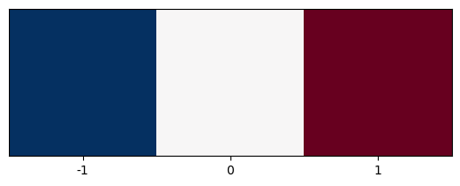
The x-gradient kernel below, is shown below, and is reminiscent of the edge-detection or sharpening kernels used in image processing and machine learning:

plt.imshow([[-1,0,1]], cmap=plt.cm.RdBu_r)
plt.xticks([0,1,2], labels=[-1,0,1]);
plt.yticks([]);

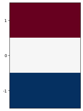
The first-order partial derivative in \(y\) is similarly discretized as:

\[\frac{\partial T(x_{i}, y_{j}, t_{n})}{\partial y} \approx \frac{T_{i,\, j+1}^{n} - T_{i,\,j-1}^{n}}{2 \Delta y}.\]

Its kernel is shown below.

plt.imshow([[-1,-1],[0,0],[1,1]], cmap=plt.cm.RdBu);
plt.xticks([]);
plt.yticks([0,1,2], labels=[1,0,-1]);

Now that we have discretized the two derivate terms, we can write out the advective tendency for computing \(T_{i, j, n+1}\) as

\[u\frac{\partial T}{\partial x} + v\frac{\partial T}{\partial y} \approx u_{i,\, j}^{n} \frac{T_{i,\, j+1}^{n} - T_{i,\,j-1}^{n}}{2 \Delta y} + v_{i,\, j}^{n} \frac{T_{i,\, j+1}^{n} - T_{i,\,j-1}^{n}}{2 \Delta y}.\]

We implement this as a the advect function. This computes the advective tendency for the \((i,j)\) grid cell.

xkernel = np.zeros((1,3))
xkernel[0, :] = np.array([-1,0,1])

ykernel = np.zeros((3,1))
ykernel[:, 0] = np.array([-1,0,1])

class OceanModel:
    
    def __init_(self,T, u, v, deltax, deltay):
        self.T = [T] 
        self.u = u
        self.v = v
        self.deltax = deltax
        self.deltay = deltay
        self.j = np.arange(0, self.T[0].shape[0])
        self.i = np.arange(0, self.T[0].shape[1])
        
    def advect(self, T):
        T_advect = np.zeros((self.j.size, self.i.size))
        
        for j in range(1, T_advect.shape[0] - 1):
            for i in range(1, T_advect.shape[1] - 1):
                T_advect[j, i] = -(self.u[j, i] * np.sum(xkernel[0, :] * T[j, i-1 : i + 2])/(2*self.deltax) +
                                   self.v[j, i] * np.sum(ykernel[:, 0] * T[j-1:j+2, i])/(2*self.deltay))
        return T_advect    

2.2) Discretizing diffusion in two dimensions

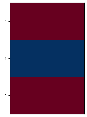
Just as with advection, the process for discretizing the diffusion operators effectively consists of repeating the one-dimensional process for \(x\) in a second dimension \(y\), separately:

\[\kappa \left( \frac{\partial^{2} T}{\partial x^{2}} + \frac{\partial^{2} T}{\partial y^{2}} \right) = \kappa \left( \frac{T_{i+1,\;j}^{n} - 2T_{i,\;j}^{n} + T_{i-1,\;j}^{n}}{\left( \Delta x \right)^{2}} + \frac{T_{i,\;j+1}^{n} - 2T_{i,\;j}^{n} + T_{i,\;j-1}^{n}}{\left( \Delta y \right)^{2}} \right)\]

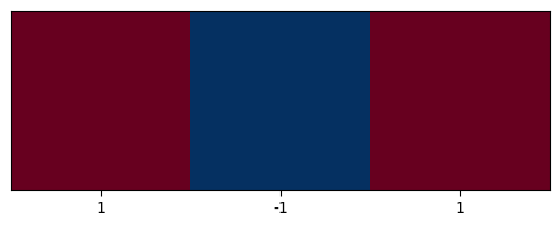
The corresponding \(x\) and \(y\) second-derivative kernels are shown below:

plt.imshow([[1,1],[0,0],[1,1]], cmap=plt.cm.RdBu_r);
plt.xticks([]);
plt.yticks([0,1,2], labels=[1,-1,1]);

plt.imshow([[1,0,1]], cmap=plt.cm.RdBu_r);
plt.xticks([0,1,2], labels=[1,-1,1]);
plt.yticks([]);

xkernel_diff = np.zeros((1, 3))
xkernel_diff[0, :] = np.array([1,-2,1])

ykernel_diff = np.zeros((3,1))
ykernel_diff[:, 0] = np.array([1,-2,1])

Just as we did with advection, we implement a diffuse function using multiple dispatch:

class OceanModel():
    
    def __init__(self, T, deltat, windfield, grid, kappa):
        
        self.T = [T]
        self.u = windfield.u
        self.v = windfield.v
        self.deltay = grid.deltay
        self.deltax = grid.deltax
        self.deltat = deltat
        self.kappa = kappa
        self.i = np.arange(0, self.T[0].shape[1])
        self.j = np.arange(0, self.T[0].shape[0])
        self.t = [0]
        self.diffuse_out = []
        self.advect_out = []
        self.t_ = []

    def advect(self, T):
        T_advect = np.zeros((self.j.size, self.i.size))
        for j in range(1, T_advect.shape[0] - 1):
            for i in range(1, T_advect.shape[1] - 1):
                T_advect[j, i] = -(self.u[j, i] * np.sum(xkernel[0, :] * T[j, i-1:i+2])/(2*self.deltax) + \
                                   self.v[j, i] * np.sum(ykernel[:, 0] * T[j-1:j+2, i])/(2*self.deltay))
        return T_advect
                
    def diffuse(self, T):
        T_diffuse= np.zeros((self.j.size, self.i.size))
        for j in range(1, T_diffuse.shape[0] - 1):
            for i in range(1, T_diffuse.shape[1] - 1):
                T_diffuse[j, i] = self.kappa*(np.sum(xkernel_diff[0, :] * T[j, i-1:i+2])/(self.deltax**2) + \
                                              np.sum(ykernel_diff[:, 0] * T[j-1:j+2, i])/(self.deltay**2))      
        return T_diffuse

2.3) No-flux boundary conditions

We want to impose the no-flux boundary conditions, which states that

\(u\frac{\partial T}{\partial x} = \kappa \frac{\partial T}{\partial x} = 0\) at \(x\) boundaries and

\(v\frac{\partial T}{\partial y} = \kappa \frac{\partial T}{\partial y} = 0\) at the \(y\) boundaries.

To impose this, we treat \(i=1\) and \(i=N_{x}\) as ghost cells, which do not do anything expect help us impose these boundaries conditions. Discretely, the boundary fluxes between \(i=1\) and \(i=2\) vanish if

\(\dfrac{T_{2,\,j}^{n} -T_{1,\,j}^{n}}{\Delta x} = 0\) or

\(T_{1,\,j}^{n} = T_{2,\,j}^{n}.\)

Thus, we can implement the boundary conditions by updating the temperature of the ghost cells to match their interior-point neighbors:

def update_ghostcells(var):
    var[0, :] = var[1, :];
    var[-1, :] = var[-2, :]
    var[:, 0] = var[:, 1]
    var[:, -1] = var[:, -2]
    return var

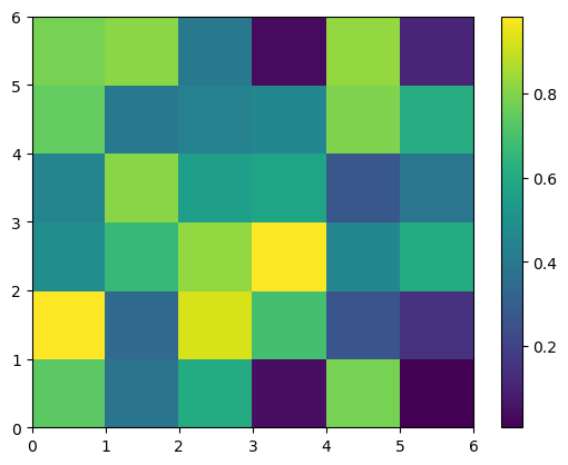
B = np.random.rand(6,6)
plt.pcolor(B)
plt.colorbar()

<matplotlib.colorbar.Colorbar at 0x13a4a7d90>

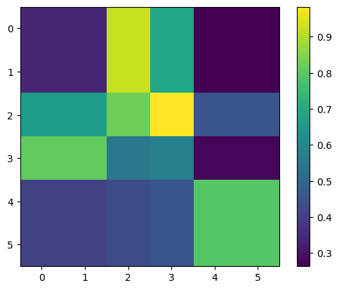
B = update_ghostcells(B)

plt.imshow(B)
plt.colorbar()

<matplotlib.colorbar.Colorbar at 0x13a537640>

2.4) Timestepping

class OceanModel():
    
    def __init__(self, T, deltat, windfield, grid, kappa):
        
        self.grid = grid
        self.T = [T]
        self.u = windfield['u']
        self.v = windfield['v']
        self.deltat = deltat
        self.kappa = kappa
        self.omega = 7.2921e-5  # Earth's angular velocity in rad/s
        self.f = 2 * self.omega * np.sin(np.deg2rad(grid.lat_grid))  # Coriolis parameter f
        self.i = np.arange(0, T.shape[1])
        self.j = np.arange(0, T.shape[0])
        self.t = [0]
        self.diffuse_out = []
        self.advect_out = []
        self.t_ = []

    def update_ghostcells(self, var):
        var[0, :] = var[1, :];
        var[-1, :] = var[-2, :]
        var[:, 0] = var[:, 1]
        var[:, -1] = var[:, -2]
        return var

    def advect(self, T):
        T_advect = np.zeros((self.j.size, self.i.size))
        for j in range(1, T_advect.shape[0] - 1):
            for i in range(1, T_advect.shape[1] - 1):
                T_advect[j, i] = -(self.u[j, i] * np.sum(xkernel[0, :] * T[j, i-1:i+2])/(2*self.grid.delta_lon[j,i]) + \
                                   self.v[j, i] * np.sum(ykernel[:, 0] * T[j-1:j+2, i])/(2*self.grid.delta_lat))
        return T_advect
                
    def diffuse(self, T):
        T_diffuse= np.zeros((self.j.size, self.i.size))
        for j in range(1, T_diffuse.shape[0] - 1):
            for i in range(1, T_diffuse.shape[1] - 1):
                T_diffuse[j, i] = self.kappa*(np.sum(xkernel_diff[0, :] * T[j, i-1:i+2])/(self.grid.delta_lon[j,i]**2) + \
                                              np.sum(ykernel_diff[:, 0] * T[j-1:j+2, i])/(self.grid.delta_lat**2))      
        return T_diffuse
    
    def timestep(self):
        T_ = self.update_ghostcells(self.T[-1].copy())
        
        # Calculate Coriolis forces
        f_u = -self.f * self.v
        f_v = self.f * self.u
        
        # Update the velocities with the Coriolis effect
        self.u += self.deltat * f_u
        self.v += self.deltat * f_v

        # Proceed with advection and diffusion as before
        tendencies = self.advect(T_) + self.diffuse(T_)
        T_ += self.deltat * tendencies

        # Store the new temperature field
        self.T.append(T_)
        self.t.append(self.t[-1] + self.deltat)

# You can instantiate the grid outside of the OceanModel like this:
N_lat = 180  # Number of latitude grid points
N_lon = 360  # Number of longitude grid points
grid = Grid(N_lat, N_lon)

# And then create the OceanModel with the new grid:
windfield = {'u': np.random.rand(N_lat, N_lon), 'v': np.random.rand(N_lat, N_lon)}

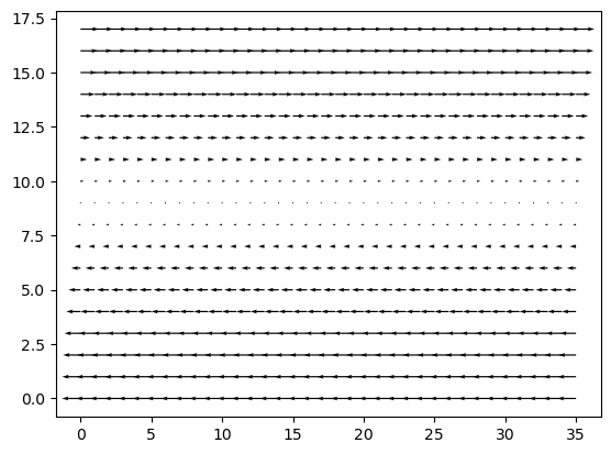
def create_wind_field(N_lat, N_lon, max_speed=10):
    """
    Create a simple zonal wind field for an aquaplanet.

    Parameters:
    N_lat -- number of latitude grid points
    N_lon -- number of longitude grid points
    max_speed -- maximum speed of the wind (m/s)

    Returns:
    windfield -- a dictionary with 'u' and 'v' components of wind
    """
    # Create a latitude array that goes from -90 to 90 degrees
    latitudes = np.linspace(-90, 90, N_lat)

    # Create the zonal wind profile - simple sinusoidal variation
    u_wind_profile = max_speed * np.sin(np.deg2rad(latitudes))

    # Create the u component of the wind field - it varies with latitude but is constant with longitude
    u_wind = np.tile(u_wind_profile, (N_lon, 1)).T

    # The v component (meridional wind) is zero in this simple model
    v_wind = np.zeros((N_lat, N_lon))

    windfield = {'u': u_wind, 'v': v_wind}

    return windfield

# Example usage:
N_lat = 180  # number of latitude points
N_lon = 360  # number of longitude points
windfield = create_wind_field(N_lat, N_lon)

kappa = 1e-6  # Example diffusivity
deltat = 3600  # Example time step in seconds

[[5.         4.99923423 4.99693714 ... 4.99693714 4.99923423 5.        ]
 [5.52649688 5.52573111 5.52343402 ... 5.52343402 5.52573111 5.52649688]
 [6.05283158 6.05206581 6.04976873 ... 6.04976873 6.05206581 6.05283158]
 ...
 [6.05283158 6.05206581 6.04976873 ... 6.04976873 6.05206581 6.05283158]
 [5.52649688 5.52573111 5.52343402 ... 5.52343402 5.52573111 5.52649688]
 [5.         4.99923423 4.99693714 ... 4.99693714 4.99923423 5.        ]]

import numpy as np
import matplotlib.pyplot as plt
import cartopy.crs as ccrs
import cartopy.feature as cfeature

# Create latitude array from -90 to 90 degrees
latitudes = np.linspace(-90, 90, N_lat)

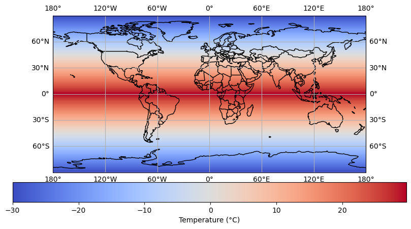
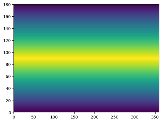
# Create an initial temperature distribution with higher temperatures at the Equator
initial_temperature = np.zeros((N_lat, N_lon))

# Assuming a simplistic temperature gradient
for i, lat in enumerate(latitudes):
    initial_temperature[i, :] = max(30 - abs(lat)/90 * 60, -30)  # Temperature decreases from equator to poles

# Set up the map projection and the figure
fig = plt.figure(figsize=(10, 5))
ax = fig.add_subplot(1, 1, 1, projection=ccrs.PlateCarree())

# Set up the longitude and latitude arrays for the grid
longitudes = np.linspace(-180, 180, N_lon)
latitudes = np.linspace(-90, 90, N_lat)

# Create a meshgrid for the map projection
lon2d, lat2d = np.meshgrid(longitudes, latitudes)

# Plot the data using pcolormesh
temperature_plot = ax.pcolormesh(lon2d, lat2d, initial_temperature, 
                                 transform=ccrs.PlateCarree(), 
                                 cmap='coolwarm')

# Add coastlines for context
ax.coastlines()

# Add a color bar
cbar = plt.colorbar(temperature_plot, orientation='horizontal', pad=0.05)
cbar.set_label('Temperature (°C)')

# Set map extent (could be global or specific region)
ax.set_global()

# Add gridlines and features
ax.gridlines(draw_labels=True, dms=True, x_inline=False, y_inline=False)
ax.add_feature(cfeature.BORDERS)

# Show the plot
plt.show()

plt.quiver(windfield["u"][::10,::10], windfield["v"][::10,::10])

<matplotlib.quiver.Quiver at 0x172090250>

model = OceanModel(initial_temperature, deltat, windfield, grid, kappa)

grid.delta_lon.shape

(180, 360)

model.timestep()

plt.pcolor(model.T[2])

<matplotlib.collections.PolyCollection at 0x28613fa90>

import numpy as np

class Grid:
    """ Creates grid for ocean model on a spherical surface (aqua planet). """
    def __init__(self, N_lat, N_lon, radius=6371e3):
        """
        Args:
        N_lat: Number of latitude grid points
        N_lon: Number of longitude grid points
        radius: Radius of the planet (default is Earth's radius in meters)
        """
        self.radius = radius
        
        # Latitude ranges from -90 to 90 degrees
        self.lat = np.linspace(-90, 90, N_lat)
        
        # Longitude ranges from -180 to 180 degrees (or 0 to 360)
        self.lon = np.linspace(-180, 180, N_lon, endpoint=False)

        # Create 2D arrays of lat and lon values
        self.lon_grid, self.lat_grid = np.meshgrid(self.lon, self.lat)
        
        # Calculate grid spacing in meters
        # Circumference at a given latitude is 2 * pi * radius * cos(latitude)
        # Grid spacing in longitude direction changes with latitude
        
        self.delta_lat = np.pi * radius / (N_lat - 1)
        self.delta_lon = (2 * np.pi * radius / N_lon) * np.cos(np.deg2rad(self.lat_grid))

        self.N_lat = N_lat
        self.N_lon = N_lon
    
    def get_coordinates(self):
        """ Get the spherical coordinates of the grid points. """
        # Convert degrees to radians for calculations
        lat_rad = np.deg2rad(self.lat_grid)
        lon_rad = np.deg2rad(self.lon_grid)
        
        # Convert lat/lon to Cartesian coordinates for a sphere
        x = self.radius * np.cos(lat_rad) * np.cos(lon_rad)
        y = self.radius * np.cos(lat_rad) * np.sin(lon_rad)
        z = self.radius * np.sin(lat_rad)
        
        return x, y, z
    
    def get_grid_spacing_meters(self):
        """ Get the grid spacing in meters for both latitude and longitude. """
        return self.delta_lat, self.delta_lon

# Example usage:
N_lat = 180  # Number of latitude grid points
N_lon = 360  # Number of longitude grid points
grid = Grid(N_lat, N_lon)

class grid:   
    """ Creates grid for ocean model
    Args:
    -------
    
    N: Number of grid points (NxN)
    L: Length of domain
    """
    def __init__(self, N, L):
        self.deltax = L / N
        self.deltay = L / N
        self.xs = np.arange(0-self.deltax/2, L+self.deltax/2, self.deltax) 
        self.ys = np.arange(-L-self.deltay/2, L+self.deltay/2, self.deltay)   

        self.N = N
        self.L = L
        self.Nx = len(self.xs)
        self.Ny = len(self.ys)
        self.grid, _= np.meshgrid(self.ys, self.xs, sparse=False, indexing='ij')
        
class windfield:
    """Calculates wind velocity
    
    Args:
    ------
    Grid: class grid()
    option: zero, or single gyre
    
    """
    
    def __init__(self, grid, option = "zero"):
        if option == "zero":
            self.u = np.zeros((grid.grid.shape))
            self.v = np.zeros((grid.grid.shape))
        if option == "single_gyre":
            u, v = PointVortex(grid)
            self.u = u
            self.v = v

import matplotlib.pyplot as plt
import cartopy.crs as ccrs
import cartopy.feature as cfeature
from ipywidgets import interact, IntSlider
import numpy as np


def plot_temperature_distribution(T, grid):
    # Create a figure with an axes set with a projection
    fig = plt.figure(figsize=(12, 6))
    ax = fig.add_subplot(1, 1, 1, projection=ccrs.PlateCarree())
    ax.add_feature(cfeature.COASTLINE)
    ax.add_feature(cfeature.BORDERS, linestyle=':')
    
    # Set the extent (min longitude, max longitude, min latitude, max latitude)

    # Plot the temperature data
    mesh = ax.pcolormesh(grid.lon_grid, grid.lat_grid, T, 
                         cmap='coolwarm', transform=ccrs.PlateCarree())
    
    # Add a colorbar
    cbar = plt.colorbar(mesh, orientation='vertical', pad=0.02, aspect=50)
    cbar.set_label('Temperature (°C)')
    
    # Add titles and labels
    plt.title('Ocean Surface Temperature')
    ax.set_xlabel('Longitude')
    ax.set_ylabel('Latitude')

    plt.show()

def update_model(steps):
    for _ in range(steps):
        model.timestep()  # Call the timestep method of your model
    plot_temperature_distribution(model.T[-1], model.grid)  # Plot the latest temperature distribution

# Initialize your model here with the initial conditions
# Example:
model = OceanModel(initial_temperature, deltat, windfield, grid, kappa)

# Create an interactive slider for number of timesteps
interact(update_model, steps=IntSlider(min=1, max=100, step=1, value=1, description='Time Steps'))

<function __main__.update_model(steps)>

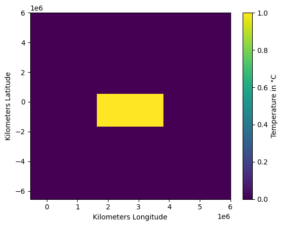
Initialize \(10x10\) grid domain with \(L=6000000m\) and a windfield, where all velocities are set to zero. This should result in diffusion only.

Initialize temperature field with rectangular non-zero box.

%matplotlib inline
import matplotlib.pyplot as plt
import cartopy.crs as ccrs
import cartopy.feature as cfeature
import numpy as np
from ipywidgets import interactive, IntSlider

# Assume your OceanModel class definition is here

def plot_temperature_distribution(model):
    fig = plt.figure(figsize=(10, 5))
    ax = fig.add_subplot(1, 1, 1, projection=ccrs.PlateCarree())
    
    # Retrieve the latest temperature data from the model
    T = model.T[-1]

    # Clear the previous plot to ensure we do not overlay the plots
    ax.clear()
    
    # Plot the temperature distribution
    temperature_plot = ax.pcolormesh(model.grid.lon_grid, model.grid.lat_grid, T, 
                                     transform=ccrs.PlateCarree(), 
                                     cmap='coolwarm')

    # Add coastlines and borders for context
    ax.coastlines()
    ax.add_feature(cfeature.BORDERS)
    
    # Add a color bar
    cbar = plt.colorbar(temperature_plot, orientation='horizontal', pad=0.05)
    cbar.set_label('Temperature (°C)')

    # Set map extent (could be global or a specific region)
    ax.set_global()
    
    # Add gridlines
    ax.gridlines(draw_labels=True, dms=True, x_inline=False, y_inline=False)
    
    # Show the plot
    plt.show()

def timestep_and_plot(steps):
    for _ in range(steps):
        model.timestep()  # Call the timestep method of your model
    plot_temperature_distribution(model)  # Plot the latest temperature distribution

# Initialize your model here with the initial conditions
# Example:
model = OceanModel(initial_temperature, deltat, windfield, grid, kappa)

# Create an interactive widget to control the number of timesteps
slider = IntSlider(min=1, max=100, step=1, value=1, description='Time Steps')
interactive_plot = interactive(timestep_and_plot, steps=slider)
display(interactive_plot)

my_grid = grid(N = 11, L = 6e6)
my_wind = windfield(my_grid, option = "zero")
my_temp = np.zeros((my_grid.grid.shape)) 
my_temp[9:13, 4:8] = 1

my_grid.grid.shape

(23, 12)

plt.pcolor(my_grid.xs, my_grid.ys, my_temp)
plt.colorbar(label = "Temperature in °C");
plt.ylabel("Kilometers Latitude");
plt.xlabel("Kilometers Longitude");

deltat = 12*60*60 # 12 Hours

def plot_func(steps, temp, deltat, windfield, grid, kappa, anomaly = False):
    my_model = OceanModel(T=temp,
                      deltat=deltat, 
                      windfield=windfield, 
                      grid=grid, 
                      kappa = kappa)
    for step in range(steps):
        my_model.timestep()   
    plt.figure(figsize=(8,8))
    lon, lat = np.meshgrid(grid.xs, grid.ys)
    if anomaly == True:
        plt.pcolor(my_grid.xs, my_grid.ys, my_model.T[-1] - my_model.T[-2], cmap = plt.cm.RdBu_r,
                  vmin = -0.001, vmax = 0.001)
    else:
        plt.pcolor(my_grid.xs, my_grid.ys, my_model.T[-1], vmin = 0, vmax = 1)
    plt.quiver(lon, lat, windfield.u, windfield.v)
    plt.colorbar(label = "Temperature in °C");
    plt.ylabel("Kilometers Latitude");
    plt.xlabel("Kilometers Longitude"); 
    plt.title("Time: {} days".format(int(step/2)))
    plt.show()

interact(plot_func, 
         temp = fixed(my_temp),
         deltat = fixed(deltat),
         windfield = fixed(my_wind),
         grid = fixed(my_grid),
         kappa = fixed(1e4),
         anomaly = widgets.Checkbox(description = "Anomaly", value=False),
         steps = widgets.IntSlider(description="Timesteps", value = 2, min = 1, max = 10000, step = 1));

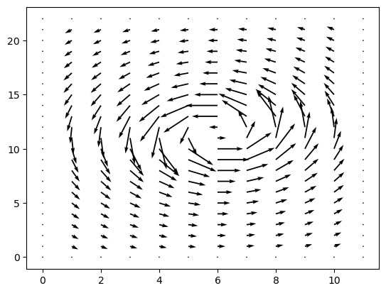
Create single gyre windfield

def diagnose_velocities(stream, G):    
    dx = np.zeros((G.grid.shape))
    dy = np.zeros((G.grid.shape))
    
    dx = (stream[:, 1:] - stream[:, 0:-1])/G.deltax
    dy = (stream[1:, :] - stream[0:-1, :])/G.deltay
    
    u = np.zeros((G.grid.shape))
    v = np.zeros((G.grid.shape))
    
    u = 0.5*(dy[:, 1:] + dy[:, 0:-1])
    v = -0.5*(dx[1:, :] + dx[0:-1, :])
    
    return u, v

def impose_no_flux(u, v):
    u[0, :]  = 0; v[0, :] = 0;
    u[-1,:]  = 0; v[-1,:] = 0;
    u[:, 0]  = 0; v[:, 0] = 0;
    u[:,-1]  = 0; v[:,-1] = 0;
    
    return u, v

def PointVortex(G, omega = 0.6, a = 0.2, x0=0.5, y0 = 0.):
    x = np.arange(-G.deltax/G.L, 1 + G.deltax / G.L, G.deltax / G.L).reshape(1, -1)
    y = np.arange(-1-G.deltay/G.L, 1+ G.deltay / G.L, G.deltay / G.L).reshape(-1, 1)
        
    r = np.sqrt((y - y0)**2 + (x - x0)**2)
    stream = -omega/4*r**2 
    stream[r > a] =  -omega*a**2/4*(1. + 2*np.log(r[r > a]/a))
    
    u, v =  diagnose_velocities(stream, G)
    u, v = impose_no_flux(u, v) 
    u = u * G.L; v = v * G.L
    return u, v

my_wind = windfield(my_grid, option="single_gyre")
plt.quiver(my_wind.u, my_wind.v)

<matplotlib.quiver.Quiver at 0x134f329b0>

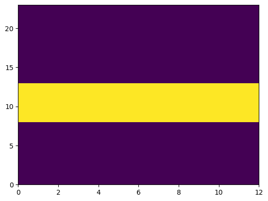
my_temp = np.zeros((my_grid.grid.shape)) 
my_temp[8:13, :] = 1

plt.pcolor(my_temp)

<matplotlib.collections.PolyCollection at 0x134f30190>

my_model = OceanModel(T=my_temp,
                      deltat=deltat, 
                      windfield=my_wind, 
                      grid=my_grid, 
                      kappa = 1e4)

interact(plot_func, 
         temp = fixed(my_temp),
         deltat = fixed(deltat),
         windfield = fixed(my_wind),
         grid = fixed(my_grid),
         kappa = widgets.IntSlider(description="kappa", value = 1e4, min=1e3, max = 1e5, step = 100),
         anomaly = widgets.Checkbox(description = "Anomaly", value=False),
         steps = widgets.IntSlider(description="Timesteps", value = 1, min = 1, max = 1000, step = 1));

Optional: Create two gyres!